11Inflation Derivatives

In October 2022 the UK retail price index stood 14.2% above its level a year earlier. Many British pension schemes do not promise their members full inflation: their increases are the index’s annual change floored at zero and capped at 5% (2.5% for rights earned since 2005). Schemes that had hedged those promises with plain index swaps held hedges that paid the whole 14.2% on liabilities that would rise by 5; the difference between an index and a capped, annually reset index had become the largest number in their risk report. Every inflation product beyond the zero-coupon swap of One Quant Book 2, chapter 11, depends on how the index moves from year to year, and that is a question for a model. This chapter builds the standard one on an analogy with foreign exchange, computes the convexity that separates year-on-year from zero-coupon products, adds seasonality, and prices limited price indexation by simulation.

11.1 The foreign-currency analogy

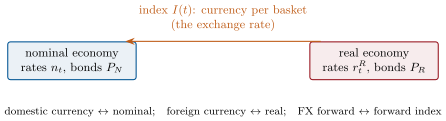
Treat nominal money as one currency and “real” money, a unit of the basket, as another. A nominal bond pays currency; an index-linked bond pays a basket, worth $I(T)$ units of currency. The index is the exchange rate between the two, real discount factors $P_R(t,T)$ are the foreign currency’s discount factors, and the forward index is a forward exchange rate:

a martingale under the nominal $T$-forward measure. A zero-coupon inflation swap fixes $(1+k_T)^T = I(0,T)/I(0)$, so today’s real curve is read from the swaps: $P_R(0,T) = P_N(0,T)(1+k_T)^T$.

The chapter keeps nominal rates deterministic, which isolates the effects of the real rate and the index; the full model adds terms in the nominal volatility and its correlations of the same form.

11.2 Zero-coupon versus year-on-year

A zero-coupon swap pays one ratio $I(T)/I(0)$ at $T$: its value needs only the forward index. A year-on-year leg pays a ratio of two future index values, paid at the later date; its value needs the expectation of the ratio under the nominal measure of the payment date, and the ratio’s numerator and denominator are correlated through the real rate.

    def yoy_ratio(self, T: float, S: float) -> float:
        """E^N[I(S) / I(T)]: the forward ratio times exp(C), C the year-on-year convexity adjustment."""
        fwd = (self.real.df_t(S) / self.real.df_t(T)) / (self.nominal.df_t(S) / self.nominal.df_t(T))
        return fwd * math.exp(self.convexity(T, S))

    def convexity(self, T: float, S: float) -> float:
        b = _B(self.kappa, S - T)
        return -b * (self.mu(T) - self.rho * self.sigma_r * self.sigma_i * _B(self.kappa, T))

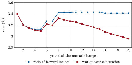
The sign and size depend on the correlation: at the tenth year the adjustment is $-20.6$, $-16.4$ and $-12.2$ basis points for $\rho = -0.5$, $0$ and $0.5$. With no real-rate volatility it vanishes whatever $\rho$; the index volatility alone does not create it.

11.3 Seasonality in the model

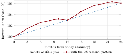
Price indices are not seasonally adjusted, and their monthly changes follow the calendar: sales, energy tariffs, holidays (One Quant Book 2, chapter 11). An inflation swap or bond references a given month’s index, so the forward index must carry the pattern between annual points while matching them.

11.4 Inflation options and limited price indexation

In the model the annual ratio is lognormal: its log-variance is the index variance over the year plus the variance of the year’s real-rate integral, less twice their covariance, and the caplet is Black’s formula on the year-on-year expectation.

Compounding capped and floored changes is path-dependent: the payoff is not a sum of caplets. It is priced by simulating the year-on-year ratios jointly.

    def lpi_leg(self, years: int, cap: float = 0.05, floor: float = 0.0, paths: int = 40000, seed: int = 11) -> dict:
        """Value at 0 of LPI(years) = prod (1 + min(max(ratio - 1, floor), cap)) paid at `years`,
        and of the uncapped index ratio I(years)/I(0)."""
        r = self.simulate_ratios(years, paths, seed=seed)
        lpi = np.prod(1 + np.clip(r - 1, floor, cap), axis=1)
        full = np.prod(r, axis=1)
        p = self.nominal.df_t(years)
        return {"lpi": p * lpi.mean(), "lpi_se": p * lpi.std(ddof=1) / math.sqrt(paths),
                "uncapped": p * full.mean(), "uncapped_exact": self.real.df_t(years)}

11.5 Tutorial: year-on-year products

11.6 Build: inflation options

11.7 Exercises

11.8 Problem: The Pension Fund’s LPI Swap

11.9 Interview questions