Rates, Credit, XVA and Risk · Rates, credit & risk

7Short-Rate Models

Every night a bank values tens of thousands of callable bonds, Bermudan swaptions and mortgage pools, each an option to exercise on one of many dates on a whole curve. A model of the swap rate alone cannot do it: exercising at year three depends on every rate from year three on. The oldest workable answer models one number, the instantaneous short rate, and derives the whole curve from it; the version most banks still run in production fits today’s curve exactly, has bond and swaption prices in closed form, and fits on a tree that values a Bermudan in milliseconds. Its limits are as well known as its uses: one factor makes every rate move together, and one volatility cannot fit the swaptions it will be asked to hedge. This chapter builds that model, the Hull–White model, fits it to chapter 2’s euro curve and to chapter 5’s co-terminal swaptions, checks its tree against its formulas, and measures what a second factor adds.

7.1 The short rate and affine bond prices

Definition 7.1 (Short-rate model)

A short-rate model specifies the dynamics of the instantaneous rate $r_t$ under the risk-neutral measure $\mathbb Q$ (One Quant Book 4, chapter 5), and prices every zero-coupon bond as $P(t,T) = \E^{\mathbb Q}_t\bigl[\exp(-\int_t^Tr_s\,ds)\bigr]$ .

Definition 7.2 (Affine term-structure model)

A short-rate model is an affine term-structure model if its bond prices are exponential-affine in the state: $P(t,T) = \exp\bigl(\mathcal A(t,T)-\mathcal B(t,T)\,x_t\bigr)$ for a state $x_t$ (the short rate or a vector of factors) and deterministic functions $\mathcal A, \mathcal B$ . By the Feynman–Kac formula (One Quant Book 4, chapter 4) this holds whenever the drift and the variance of the state are affine in it.

Definition 7.3 (Vasicek model)

The Vasicek model (1977) makes the short rate an Ornstein–Uhlenbeck process, $dr_t = \kappa(\bar x-r_t)\,dt+\sigma\,dW_t$ : mean reversion at speed $\kappa$ to a level $\bar x$ , normal increments, negative rates possible.

Proposition 7.4 (Vasicek bond prices)

With $B(\tau) = (1-e^{-\kappa\tau})/\kappa$ ,

P(t,T) = \exp\Bigl(\bigl(\bar x-\tfrac{\sigma^2}{2\kappa^2}\bigr)\bigl(B(\tau)-\tau\bigr) -\tfrac{\sigma^2}{4\kappa}B(\tau)^2 - B(\tau)\,r_t\Bigr),\qquad \tau = T-t,

and the long zero rate tends to $\bar x-\sigma^2/(2\kappa^2)$ : convexity pulls long yields below the mean level.

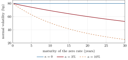
Proof. $\int_t^Tr_s\,ds$ is normal given $r_t$ , with mean $\bar x\tau+(r_t-\bar x)B(\tau)$ and variance $\frac{\sigma^2}{\kappa^2}\bigl(\tau-B(\tau)-\frac\kappa2 B(\tau)^2\bigr)$ ; take $\E[e^{-X}] = e^{-\E X+\Var X/2}$ . ∎

A one-factor Gaussian model gives every zero rate $z(t,T) = -\ln P/\tau$ the normal volatility $\sigma B(\tau)/\tau$ . Mean reversion is thus the model’s knob for the shape of the volatility curve, not a statement about where rates are going: with $\kappa=0$ every zero rate has the same volatility, and with $\kappa>0$ long rates are less volatile than short ones (Figure 7.1).

Normal volatility of zero rates, B( )/, in a one-factor Gaussian model with = 80 basis points: mean reversion damps the volatility of long rates (69.1 basis points at ten years with =3\%, 50.6 with =10\%). Data: the chapter’s tutorial. — **Figure 7.1.** Normal volatility of zero rates, $\sigma B(\tau)/\tau$ , in a one-factor Gaussian model with $\sigma = 80$ basis points: mean reversion damps the volatility of long rates (69.1 basis points at ten years with $\kappa=3\%$ , 50.6 with $\kappa=10\%$ ). Data: the chapter’s tutorial.

7.2 Vasicek and Hull–White

Vasicek’s model has three parameters and cannot fit today’s curve. Hull and White made the level time-dependent and chose it to fit.

Definition 7.5 (Hull–White model)

The Hull–White model (1990) is $dr_t = (\vartheta(t)-\kappa r_t)\,dt+\sigma(t)\,dW_t$ with $\vartheta(t)$ chosen so that the model’s bond prices equal today’s discount factors for every maturity. Equivalently, $r_t = f(0,t)+x_t$ with

dx_t = \bigl(y(t)-\kappa x_t\bigr)dt+\sigma(t)\,dW_t,\quad x_0=0,\qquad y(t) = \int_0^te^{-2\kappa(t-u)}\sigma(u)^2\,du .

Proposition 7.6 (Hull–White bonds and bond options)

With $B(t,T) = (1-e^{-\kappa(T-t)})/\kappa$ ,

P(t,T) = \frac{P(0,T)}{P(0,t)}\exp\Bigl(-B(t,T)\,x_t-\tfrac12B(t,T)^2y(t)\Bigr),

so $\ln P(T,S)$ is normal with standard deviation $\sigma_P = B(T,S)\sqrt{y(T)}$ , and a call at $T$ on the bond maturing at $S$ , strike $K$ , is worth $P(0,S)\Phi(h)-KP(0,T)\Phi(h-\sigma_P)$ with $h = \ln\frac{P(0,S)}{KP(0,T)}/\sigma_P+\sigma_P/2$ .

Proof. Admitted here. ∎

(a Gaussian computation under the $T$ -forward measure; Brigo and Mercurio, 2006, chapter 3.)

Definition 7.7 (Black–Karasinski model)

The Black–Karasinski model (1991) makes the logarithm of the short rate mean-reverting and normal, $d\ln r_t = (\vartheta(t)-\kappa\ln r_t)\,dt+\sigma\,dW_t$ : rates stay positive, bond prices have no closed form, and the model is used on trees. It lost ground when rates went negative.

7.3 Calibration to the curve and to swaptions

The curve is fitted by construction. The volatility must be fitted to options, and the options that matter are those the product can be exercised into: for a ten-year Bermudan callable every year, the co-terminal swaptions, one year into nine, two into eight, up to nine into one.

Definition 7.8 (Jamshidian decomposition)

The Jamshidian decomposition (1989) writes an option on a coupon bond, in a one-factor model where every bond price at expiry is a decreasing function of the single state $x_T$ , as a portfolio of options on its zero-coupon bonds: with $x^\star$ the state at which the coupon bond is worth the strike, each zero-coupon option is struck at that bond’s price at $x^\star$ .

A receiver swaption with strike $K$ is a call at par on a bond paying $K$ each year and one at maturity, so it is a sum of zero-coupon bond calls priced by Proposition 7.6.

    def swaption(self, T: float, tenor: int, K: float, payer: bool = True) -> float:
        """European swaption (annual unit accruals) by Jamshidian's decomposition: the receiver is a
        call on a coupon bond, i.e. a portfolio of calls on zero-coupon bonds struck at P(T, t_i; x*)."""
        pay = [T + i for i in range(1, tenor + 1)]
        cf = [K] * tenor
        cf[-1] += 1.0

        yt = self.y(T)

        def bond_value(x):
            return sum(c * self.bond(T, t, x, yt) for c, t in zip(cf, pay, strict=True))
        lo, hi = -1.0, 1.0
        for _ in range(100):
            mid = 0.5 * (lo + hi)
            lo, hi = (mid, hi) if bond_value(mid) > 1.0 else (lo, mid)
        xs = 0.5 * (lo + hi)
        return sum(c * self.zbo(T, t, self.bond(T, t, xs, yt), call=not payer) for c, t in zip(cf, pay, strict=True))

Listing 7.1. European swaptions in Hull–White by Jamshidian’s decomposition. code/firm/shortrate/firm_shortrate.py

Method 7.9 (Co-terminal calibration)

Fix $\kappa$ (it shapes the volatility term structure; it is often set from the ratio of volatilities of different tenors, or by desk convention). For the co-terminal expiries $e_1<\dots<e_m$ into a common final date, take $\sigma(t)$ piecewise constant on $[e_{i-1},e_i)$ and solve for each level in turn so that the at-the-money swaption expiring at $e_i$ reprices at its market volatility, the earlier levels held. Check the resulting $\sigma(t)$ for smoothness and sign.

Example 7.10 (One sigma is not enough)

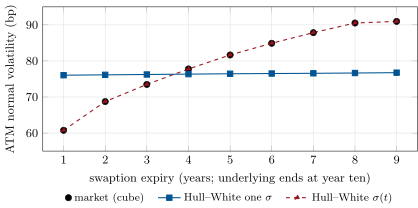
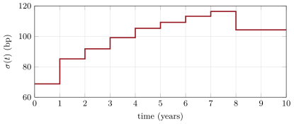
On chapter 2’s euro OIS curve with $\kappa=3\%$ , the co-terminal swaptions into ten years from chapter 5’s cube have at-the-money normal volatilities from 60.8 basis points (one into nine) to 91.0 (nine into one). The best constant $\sigma$ , 86.0 basis points, gives model volatilities between 76.0 and 76.7: it misses the one-year expiry by 15.3 basis points and the nine-year by 14.2 (Figure 7.2). A piecewise-constant $\sigma(t)$ fits all nine exactly, rising from 68.7 to 116.3 basis points before falling to 104.2 in the last interval (Figure 7.3).

Co-terminal swaptions into year ten: market volatilities and Hull–White fits with =3\%. One volatility gives an almost flat line through the middle; a piecewise-constant volatility reprices every point. Data: chapter 2’s curve and chapter 5’s synthetic cube; the chapter’s tutorial. — **Figure 7.2.** Co-terminal swaptions into year ten: market volatilities and Hull–White fits with $\kappa=3\%$ . One volatility gives an almost flat line through the middle; a piecewise-constant volatility reprices every point. Data: chapter 2’s curve and chapter 5’s synthetic cube; the chapter’s tutorial.

The piecewise-constant Hull–White volatility that reprices the nine co-terminal swaptions. It must rise to make later expiries more volatile than mean reversion alone would, a sign that =3\% and the cube’s term structure disagree. Data: the chapter’s tutorial. — **Figure 7.3.** The piecewise-constant Hull–White volatility that reprices the nine co-terminal swaptions. It must rise to make later expiries more volatile than mean reversion alone would, a sign that $\kappa=3\%$ and the cube’s term structure disagree. Data: the chapter’s tutorial.

7.4 Trees

A Bermudan swaption needs the value of continuing at each exercise date, in every state: backward induction on a lattice. The trinomial tree of One Quant Book 5, chapter 22, is built here for the Hull–White state.

Method 7.11 (The Hull–White tree)

(1) Build a tree for $x$ with $dx = -\kappa x\,dt+\sigma\,dW$ : steps $\Delta t$ , spacing $\Delta x = \sigma\sqrt{3\Delta t}$ , nodes $j\Delta x$ for $|j|\le j_{\max} = \lceil0.184/(\kappa\Delta t)\rceil$ , three branches from each node with probabilities that match the mean $-\kappa j\Delta x\Delta t$ and the variance $\sigma^2\Delta t$ , the branching shifted inwards at $\pm j_{\max}$ . (2) Shift the tree by $\alpha_i$ at each step so that it reprices the curve: carry the Arrow–Debreu prices $Q_{i,j}$ forward and set $\alpha_i = \frac1{\Delta t}\ln\bigl(\sum_j Q_{i,j}e^{-j\Delta x\Delta t}/P(0,t_{i+1})\bigr)$ . The short rate at node $(i,j)$ is $\alpha_i+j\Delta x$ .

        q = np.zeros(2 * jmax + 1)
        q[jmax] = 1.0
        width = [min(i, jmax) for i in range(n + 1)]
        for i in range(n + 1):
            p_next = curve.df_t((i + 1) * dt)
            ws = width[i]
            idx = np.arange(jmax - ws, jmax + ws + 1)
            s = np.sum(q[idx] * np.exp(-js[idx] * dx * dt))
            self.alpha[i] = math.log(s / p_next) / dt
            if i == n:
                break
            disc = np.exp(-(self.alpha[i] + js * dx) * dt)
            qn = np.zeros_like(q)
            for jj in idx:
                c = jj + k[jj]
                w = q[jj] * disc[jj]
                qn[c + 1] += w * self.pu[jj]
                qn[c] += w * self.pm[jj]
                qn[c - 1] += w * self.pd[jj]
            q = qn
        self.js, self.width = js, width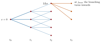

Listing 7.2. Fitting the tree to the curve by forward induction of Arrow–Debreu prices. code/firm/shortrate/firm_shortrate.py

A Hull–White trinomial tree: three branches from each node, spacing x= √3 t; once the width reaches j_ the outer nodes branch inwards, which is how the tree represents mean reversion. The short rate at each node is its x plus the step’s _i. — **Figure 7.4.** A Hull–White trinomial tree: three branches from each node, spacing $\Delta x=\sigma\sqrt{3\Delta t}$ ; once the width reaches $j_{\max}$ the outer nodes branch inwards, which is how the tree represents mean reversion. The short rate at each node is its $x$ plus the step’s $\alpha_i$ .

Example 7.12 (Tree against formula)

With $\sigma = 80$ basis points and $\kappa=3\%$ , the at-the-money five-into-five payer (forward 2.933%, annuity 4.102) is worth 0.026018 per unit notional by Jamshidian’s formula. The tree with monthly steps gives 0.026119, with fortnightly steps 0.026079, with steps of a week 0.026044 and of half a week 0.026016: the error falls roughly in proportion to the step. The ten-year discount factor is repriced exactly at every step size, by construction.

7.5 Two factors, and what one factor cannot do

In any one-factor model every rate is a function of the same state, so changes of all rates are perfectly correlated. Daily changes of the two- and ten-year Treasury yields had a correlation of 0.769 over 2016–2026 (chapter 6); a product paying on the difference of two rates (a CMS spread, chapter 6) is worthless to a one-factor model.

Definition 7.13 (Two-factor Gaussian model)

The two-factor Gaussian model (G2++) sets $r_t = \varphi(t)+x_t+y_t$ with $dx = -\kappa_1x\,dt+\sigma_1dW^1$ , $dy = -\kappa_2y\,dt+\sigma_2dW^2$ , $d\langle W^1,W^2\rangle = \rho\,dt$ , and $\varphi$ fitted to the curve. The correlation of changes of the zero rates of maturities $\tau_1$ and $\tau_2$ is

\frac{\sum_{a,b}b_a(\tau_1)b_b(\tau_2)c_{ab}}{\sqrt{\sum_{a,b}b_a(\tau_1)b_b(\tau_1)c_{ab}\,\sum_{a,b}b_a(\tau_2)b_b(\tau_2)c_{ab}}}, \quad b_a(\tau)=\frac{B(\kappa_a,\tau)}{\tau},

with $c_{11}=\sigma_1^2$ , $c_{22}=\sigma_2^2$ , $c_{12}=c_{21}=\rho\sigma_1\sigma_2$ .

Example 7.14 (Decorrelating the curve)

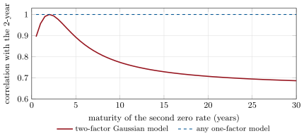
With a slow factor ( $\kappa_1=2\%$ , $\sigma_1=75$ basis points), a fast one ( $\kappa_2=50\%$ , $\sigma_2=90$ basis points) and $\rho=-0.8$ , the model’s correlation between the two- and ten-year zero rates is 0.774, close to the Treasury estimate, and between the two- and thirty-year 0.687 (Figure 7.5). The strongly negative $\rho$ is typical: the fast factor moves the front against the slow factor to produce slope moves.

Correlation of instantaneous changes of the two-year zero rate with zero rates of other maturities: one in any one-factor model, decaying with maturity in the two-factor model of . Data: the chapter’s tutorial. — **Figure 7.5.** Correlation of instantaneous changes of the two-year zero rate with zero rates of other maturities: one in any one-factor model, decaying with maturity in the two-factor model of Example 7.14. Data: the chapter’s tutorial.

7.6 Tutorial: Hull–White from curve to tree

Goal. Fit Hull–White to a curve and to co-terminal swaptions, and check its tree against its closed form. End state: Figures 7.2 and 7.3 and the numbers of Example 7.12.

The model: HullWhite(curve, kappa, sigmas, knots) reprices every discount factor of chapter 2’s €STR curve.
Calibrate: calibrations() fits one $\sigma$ and a piecewise-constant $\sigma(t)$ to the nine co-terminals; fit_table() converts model prices back to normal volatilities.
Tree: tree_check(dt=…) for monthly to half-weekly steps.
Two factors: g2_table(); fig_rc_shortrate.py writes the charts.

What to change next. Calibrate with $\kappa=0$ and $\kappa=10\%$ and compare the shapes of $\sigma(t)$ ; add a time-dependent $\sigma$ to the tree by varying the step size.

7.7 Build: the short-rate engine

Purpose. The model behind the book’s callable products: Bermudans (chapter 9), mortgages (chapter 12), exposure simulation (chapter 17).

Interface. HullWhite(curve, kappa, sigmas, knots) with bond, bond_vol, zbo, swaption, annuity_forward; calibrate_coterminal; HWTree(curve, kappa, sigma, horizon, dt) with step_back, zero_bonds_at, european_swaption; vasicek_bond, zero_rate_vol, g2_correlation.

Rules. The curve is any object with df_t; swaps with annual unit accruals in model time; numpy only.

Acceptance tests. code/firm/shortrate/tests/: bonds reprice the curve and bond options satisfy parity; payer minus receiver is the forward swap; the tree reprices discount factors and converges to Jamshidian’s price as the step shrinks; the piecewise calibration reprices its targets; Vasicek’s long rate is $\bar x-\sigma^2/2\kappa^2$ ; G2++ with one factor switched off has correlation one.

Stretch. A time-dependent $\sigma$ on the tree; a G2++ swaption formula; calibration of $\kappa$ to the ratio of co-terminal and column volatilities.

Sources and further reading

O. Vasicek, “An equilibrium characterization of the term structure”, Journal of Financial Economics 5(2), 1977.
J. Hull and A. White, “Pricing interest-rate-derivative securities”, Review of Financial Studies 3(4), 1990.
F. Jamshidian, “An exact bond option formula”, Journal of Finance 44, 1989.
F. Black and P. Karasinski, “Bond and option pricing when short rates are lognormal”, Financial Analysts Journal 47(4), 1991.
D. Brigo and F. Mercurio, Interest Rate Models: Theory and Practice, 2nd ed., Springer, 2006, chapters 3–4.

7.8 Exercises

Exercise 7.1 ★

In a one-factor Gaussian model with $\sigma = 80$ basis points and $\kappa = 3\%$ , what is the normal volatility of the ten-year and of the thirty-year zero rate?

Solution

Solution of Exercise 7.1.

$\sigma B(\tau)/\tau$ : at ten years $80\times(1-e^{-0.3})/0.3 = 69.1$ basis points; at thirty years $80\times(1-e^{-0.9})/0.9 = 52.7$ .

Exercise 7.2 ★

Why can Vasicek’s model not reprice today’s curve, and what does Hull–White change to fix it?

Solution

Solution of Exercise 7.2.

Its bond prices depend on three constants ( $\kappa$ , $\bar x$ , $\sigma$ ) and today’s short rate, a three-parameter family of curves that cannot match an arbitrary curve. Hull–White makes the drift’s level a function of time, $\vartheta(t)$ , chosen so that every discount factor is repriced; in the Gaussian form it is $r_t = f(0,t)+x_t$ .

Exercise 7.3 ★

In a Vasicek model with $\bar x = 3\%$ , $\sigma = 1\%$ and $\kappa = 10\%$ , what is the long-maturity zero rate?

Solution

Solution of Exercise 7.3.

$\bar x-\sigma^2/(2\kappa^2) = 3\%-0.0001/0.02 = 2.50\%$ .

Exercise 7.4 ★★

For the tree with monthly steps and $\kappa=3\%$ , compute $j_{\max}$ and the number of nodes at the widest step. How does it change with weekly steps?

Solution

Solution of Exercise 7.4.

$j_{\max} = \lceil0.184/(0.03/12)\rceil = 74$ : 149 nodes. With weekly steps $\lceil0.184/(0.03/52)\rceil = 319$ : 639 nodes. Small $\kappa$ makes wide trees; the width is reached only after $j_{\max}$ steps, so short trees stay narrower.

Exercise 7.5 ★★

Explain why Jamshidian’s decomposition fails in a two-factor model.

Solution

Solution of Exercise 7.5.

It needs every bond price at expiry to be a monotone function of one state variable, so that one critical value $x^\star$ splits the exercise region. With two factors the exercise boundary is a curve in the $(x,y)$ plane, and the coupon bond’s exercise region does not decompose into zero-coupon regions with a common boundary.

Exercise 7.6 ★★

Read Figure 7.3. What would the calibrated $\sigma(t)$ look like with $\kappa=10\%$ , and why?

Solution

Solution of Exercise 7.6.

Steeper: stronger mean reversion damps the volatility of long rates more, so to reproduce later expiries into shorter swaps (whose volatility the market keeps high) $\sigma(t)$ must rise faster; with a larger $\kappa$ the fit can even require large late volatilities. $\kappa$ and $\sigma(t)$ trade off: the term structure of volatility is shared between them.

Exercise 7.7 ★★★

Coding. With tree_check, tabulate the tree’s error against Jamshidian’s price for monthly, fortnightly, weekly and half-weekly steps, and estimate the order of convergence.

Solution

Solution of Exercise 7.7.

Errors against 0.026018: $+1.0\times10^{-4}$ (monthly), $+6.1\times10^{-5}$ (fortnightly), $+2.6\times10^{-5}$ (weekly), $-0.2\times10^{-5}$ (half-weekly). Halving the step roughly halves the error until it changes sign: first order, as expected for a tree whose payoff has a kink at the strike.

Exercise 7.8 ★★★

Find the flaw. “Our one-factor Hull–White model reprices every co-terminal swaption, so it prices our CMS spread options correctly.” Correct it.

Solution

Solution of Exercise 7.8.

Repricing co-terminals fixes the volatility of each swap rate; a CMS spread option also needs the correlation between the ten-year and the two-year rate, which is one in any one-factor model: the spread’s volatility collapses and the option is badly underpriced. Use a two-factor model, or a copula of the two rates’ smiles, calibrated to a correlation.

7.9 Problem: One Sigma Is Not Enough

Problem 7.1

Weekend problem — calibrating a production Hull–White model

A bank’s overnight batch prices ten-year euro Bermudans callable every year with Hull–White, $\kappa=3\%$ , on chapter 2’s €STR curve. The model validator asks why the front office uses a piecewise-constant $\sigma(t)$ when the documentation says “Hull–White with one volatility”.

Part I — The market.

Which swaptions should the model fit, and why those?
Give their volatility range and its shape.
What does a rising co-terminal volatility say about forward volatility?
Why is the curve not a calibration target?
Why is $\kappa$ fixed rather than fitted?

Part II — One sigma.

Give the best constant $\sigma$ .
Give the model’s volatility range.
Give the errors at one and nine years.
Which exercises of the Bermudan are overpriced, which underpriced?
Why can no single $\sigma$ fix it with $\kappa=3\%$ ?

Part III — Piecewise sigma.

Give the first and highest levels of $\sigma(t)$ .
Why does it fall in the last interval?
Does the fitted model price the co-terminals exactly? Other swaptions?
What does it assume about volatility beyond year nine?
What is the risk of fitting nine numbers every day?

Part IV — Judgement.

What would you write in the model documentation?
Which test would convince the validator?
What would a two-factor model add for this product, and what would it cost?
State the named result: the errors with one $\sigma$ and the range of the calibrated $\sigma(t)$ .
In one sentence: what does a production short-rate model need to fit?

Solution

Solution of Problem 7.1.

1. The co-terminals into year ten: they are the Europeans the Bermudan can be exercised into, and its value lies between the largest of them and a price that depends on their joint dynamics. 2. 60.8 to 91.0 basis points, rising with expiry. 3. That the rate volatility expected later (for shorter remaining swaps) is higher than mean reversion with a flat $\sigma$ would give. 4. The model reprices it by construction through $\vartheta(t)$ . 5. It is poorly identified from one column of co-terminals; it trades off with $\sigma(t)$ . Desks fix it by convention or from the relation between co-terminal and other swaption volatilities, and keep it stable. 6. 86.0 basis points. 7. 76.0 to 76.7 basis points. 8. $+15.3$ basis points at one year, $-14.2$ at nine years. 9. Early exercises are overpriced (the model’s short expiries are too volatile), late ones underpriced. 10. With $\kappa=3\%$ and constant $\sigma$ , co-terminal volatilities are nearly flat in expiry, while the market’s rise by 30 basis points. 11. 68.7 basis points in the first year, 116.3 at the highest (years seven to eight). 12. The last co-terminal (nine into one) has a volatility of 91.0 only slightly above the eight-year’s; to reprice it with the earlier levels held, the last interval needs less. 13. Exactly the co-terminals; other swaptions only as far as $\kappa$ and the fitted $\sigma(t)$ happen to reproduce them. 14. That it stays at the last level, 104.2 basis points. 15. Noisy parameters and P&L jumps from day to day; hedge ratios that change with the calibration rather than the market. Smooth or regularise, and monitor the parameters. 16. Hull–White with $\kappa$ fixed at 3% and a piecewise-constant $\sigma(t)$ on the co-terminal expiries, fitted daily to the co-terminal at-the-money swaptions; its limits: one factor, flat smile, no fit to other swaptions. 17. Show the co-terminal fit errors with one and with nine volatilities, the stability of $\sigma(t)$ over past months, and the Bermudan’s price under both, against a benchmark model (a market model, chapter 8). 18. Imperfect correlation between the rates exercised into, which lowers the switch value between exercise dates; the cost is slower pricing, more parameters and a correlation to mark. 19. Named result: one sigma is not enough: the best constant volatility misses the co-terminals by $+15.3$ basis points at one year and $-14.2$ at nine; the fitted $\sigma(t)$ runs from 68.7 to 116.3 basis points. 20. The curve exactly and the volatilities of the options the product can become.

7.10 Interview questions

Interview question 7.1 ★ researcher, bank

What does mean reversion do in the Hull–White model, in terms a trader would use?

Solution

Solution of Interview question 7.1.

It pulls the short rate back towards its path, so shocks to it die out and long rates move less than short ones: it sets how volatility decreases with maturity ( $\sigma B(\tau)/\tau$ ), and how correlated the exercises of a Bermudan are. A trader reads it as the model’s slope of volatility across tenors.

What the interviewer is looking for: mean reversion as a volatility-shape parameter.

Interview question 7.2 ★★ researcher

Derive the zero-coupon bond price in the Vasicek model.

Solution

Solution of Interview question 7.2.

$r$ is Ornstein–Uhlenbeck; $\int_t^Tr_s\,ds$ given $r_t$ is normal with mean $\bar x\tau+(r_t-\bar x)B(\tau)$ and variance $\frac{\sigma^2}{\kappa^2}(\tau-B-\frac\kappa2B^2)$ ; so $P = \exp(-\text{mean}+\text{variance}/2)$ , an exponential-affine function of $r_t$ .

What the interviewer is looking for: Gaussian integral and the affine form.

Interview question 7.3 ★★ researcher, developer

How do you fit a trinomial tree to today’s discount curve?

Solution

Solution of Interview question 7.3.

Build the tree for the zero-mean state first; then step forward, carrying the Arrow–Debreu prices of each node; at each step choose the shift $\alpha_i$ so that the sum of Arrow–Debreu prices times one-step discount factors equals the curve’s discount factor to the next date; update the Arrow–Debreu prices with the branching probabilities and the shifted rates.

What the interviewer is looking for: forward induction with Arrow–Debreu prices.

Interview question 7.4 ★★ trader, researcher

Which swaptions do you calibrate a one-factor model to for a ten-year Bermudan, and why not the whole matrix?

Solution

Solution of Interview question 7.4.

The co-terminal swaptions (each exercise date into the swap to the final date), because the Bermudan is exactly one of them once exercised; a one-factor model cannot fit the whole matrix, and fitting instruments the product never becomes spends parameters on irrelevant risks.

What the interviewer is looking for: the replication logic of the calibration set.

Interview question 7.5 ★★★ researcher, risk

What can a one-factor model not price, and how do you know when it matters?

Solution

Solution of Interview question 7.5.

Products depending on imperfect correlation between rates: spread options, curve-steepener exotics, and to a lesser degree Bermudans (switch value). Test by pricing with a two-factor model calibrated to the same instruments and measuring the difference; if it matters, use the richer model or reserve.

What the interviewer is looking for: correlation, and a benchmark to measure it.

Interview question 7.6 ★★★ developer

Your tree price of a European swaption differs from the closed form by 0.5%. How do you find out why?

Solution

Solution of Interview question 7.6.

Check the tree reprices discount factors (the $\alpha$ fit); halve the step and see if the error halves (discretisation) or stays (a bug); compare zero-coupon bond options with the closed form; check the exercise date and schedule alignment with the tree’s grid, the branching at the edges and the probabilities (all in $[0,1]$ , summing to one).

What the interviewer is looking for: convergence study and component tests.

Terms defined in this chapter

See all 2333 terms in the glossary