Rates, Credit, XVA and Risk · Rates, credit & risk

21Market-Risk Measures

In October 1994 J.P. Morgan published RiskMetrics: a method for turning a trading firm’s positions into one number, the loss it should not exceed on more than one day in twenty (or a hundred), together with the daily volatilities and correlations needed to compute it, free of charge. Two years later the Basel Committee let banks set their market-risk capital from their own version of the number, provided they checked it every day against what actually happened. Value at risk became the language of risk limits, capital and disclosure, and its weaknesses became as well known: it says nothing about the size of the losses beyond it, it can reward concentration, and its estimates lag the markets it measures. This chapter opens Part IV by computing the number three ways on a real book and real data, replacing it with expected shortfall, backtesting both, and allocating them to their sources.

21.1 Loss distributions and value at risk

Definition 21.1 (Risk factor)

A risk factor is a market variable whose changes drive the value of positions: a yield at a tenor, an exchange rate, an implied volatility, a credit spread. A risk model describes the joint distribution of risk-factor changes over a horizon and revalues the positions under them.

Definition 21.2 (Value at risk)

The value at risk of a portfolio at confidence level $\alpha$ over a horizon $h$ is the $\alpha$ -quantile of its loss $L = -\Delta V$ over $h$ : $\mathrm{VaR}_\alpha = \inf\{\ell:\P(L>\ell)\le1-\alpha\}$ . At 99% over one day it is a loss exceeded on one day in a hundred.

Example 21.3 (The book)

A small USD book on 23 September 2026: long USD 200 million of a ten-year Treasury par bond, short USD 300 million of a two-year, long EUR 100 million, short JPY 5 billion, and short a three-month at-the-money EURUSD straddle on EUR 400 million (implied volatility 8%, held fixed). Its four risk factors are the daily changes in the two- and ten-year par yields (4.85% and 5.11% that day) and the log returns of EURUSD (1.1411) and USDJPY (157.92). Their EWMA daily volatilities are 6.4 and 5.7 basis points, 0.28% and 0.65%.

21.2 Value at risk three ways

Definition 21.4 (Historical simulation)

Historical simulation applies each of the last $n$ observed risk-factor changes to today’s positions, revalues, and reads VaR from the empirical distribution of the $n$ P&Ls: with $k = \lceil(1-\alpha)n\rceil$ , the $k$ -th largest loss.

Definition 21.5 (Parametric value at risk)

Parametric value at risk (delta-normal) linearises the P&L in the factor changes, $\Delta V\approx\delta^\top x$ , assumes $x$ normal with covariance $\Sigma$ , and gives $\mathrm{VaR}_\alpha = z_\alpha\sqrt{\delta^\top\Sigma\delta}$ . With exponentially weighted covariances ( $\Sigma_t = \lambda\Sigma_{t-1}+(1-\lambda)x_tx_t^\top$ , $\lambda = 0.94$ for daily data in RiskMetrics) it follows volatility quickly.

Definition 21.6 (Monte Carlo value at risk)

Monte Carlo value at risk simulates factor changes from a model (here normal with the EWMA covariance), revalues the portfolio fully on each draw, and reads the quantile.

Definition 21.7 (Filtered historical simulation)

Filtered historical simulation rescales each past factor change by the ratio of today’s volatility estimate to the estimate on its day, $\tilde x_s = x_s\,\hat\sigma_{\text{today}}/\hat\sigma_s$ , before applying it: it keeps the historical shapes and dependence of the moves and today’s volatility level.

Definition 21.8 (Delta–gamma approximation)

The delta–gamma approximation replaces full revaluation by the second-order expansion $\Delta V\approx\delta^\top x+\tfrac12x^\top\Gamma x$ , with the first and second derivatives of the portfolio in the risk factors.

Example 21.9 (One book, several numbers)

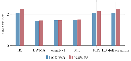
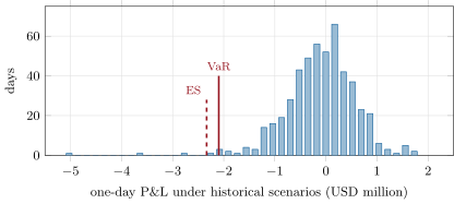
Over the last 500 days, historical simulation gives a one-day 99% VaR of USD 2.10 million; the EWMA delta-normal VaR is 1.58 million, the equal-weighted one 1.60 million, Monte Carlo with full revaluation on the EWMA covariance 1.66 million, and filtered historical simulation 2.09 million (Figure 21.1). Historical simulation with delta–gamma revaluation gives 2.10 million, delta alone 1.91: the short straddle’s gamma adds losses in both tails. The normal methods are lower because the historical moves have fatter tails than the normal.

def hs_var_es(pnl: np.ndarray, alpha: float) -> tuple[float, float]:
    losses = np.sort(-np.asarray(pnl))[::-1]
    k = max(1, math.ceil((1.0 - alpha) * len(losses) - 1e-9))
    return float(losses[k - 1]), float(losses[:k].mean())


def ewma_cov(x: np.ndarray, lam: float = 0.94) -> np.ndarray:
    """EWMA covariance of the rows of x (oldest first), zero mean, weights normalised."""
    n = x.shape[0]
    w = (1 - lam) * lam ** np.arange(n - 1, -1, -1)
    w = w / w.sum()
    return (x * w[:, None]).T @ x


def ewma_vol_path(x: np.ndarray, lam: float = 0.94, seed_obs: int = 20) -> np.ndarray:
    """EWMA volatility of each column before each observation (sigma_t uses returns up to t-1)."""
    v = np.empty_like(x)
    s2 = x[:seed_obs].var(axis=0) + 1e-18
    for t in range(x.shape[0]):
        v[t] = np.sqrt(s2)
        s2 = lam * s2 + (1 - lam) * x[t] ** 2
    return v, np.sqrt(s2)


def fhs_scenarios(x: np.ndarray, lam: float = 0.94) -> np.ndarray:
    """Filtered historical scenarios: each past return rescaled by (current vol / vol then)."""
    past, now = ewma_vol_path(x, lam)
    return x / past * now

Listing 21.1. Historical VaR and ES, EWMA covariance and volatility, and filtered historical scenarios. code/firm/varmodel/firm_varmodel.py

Definition 21.10 (Square-root-of-time rule)

The square-root-of-time rule scales a one-day VaR to $h$ days by $\sqrt h$ : exact for independent, identically distributed normal changes with zero mean and fixed positions, an approximation otherwise.

21.3 Expected shortfall and coherence

Definition 21.11 (Expected shortfall)

The expected shortfall at level $\alpha$ is the average loss in the worst $1-\alpha$ of outcomes, $\mathrm{ES}_\alpha = \frac1{1-\alpha}\int_\alpha^1\mathrm{VaR}_u\,du$ ; historically, the average of the $k$ largest losses.

Definition 21.12 (Coherent risk measure)

A risk measure $\rho$ is a coherent risk measure if it is monotone, translation invariant ( $\rho(L+c) = \rho(L)+c$ ), positively homogeneous ( $\rho(\lambda L) = \lambda\rho(L)$ for $\lambda\ge0$ ) and subadditive ( $\rho(L_1+L_2)\le\rho(L_1)+\rho(L_2)$ ). Expected shortfall is coherent; VaR is not subadditive in general.

Example 21.13 (Two concentrated bonds)

Each of two bonds defaults independently with probability 0.9%, losing 100. Each alone has a 99% VaR of zero; together, the probability of at least one default is 1.79%, so the 99% VaR is 100: diversifying raised VaR. Expected shortfall at 99% is 90 for each bond and 100.8 for the pair, less than their sum of 180.

For normal P&L, ES at 97.5% equals VaR at 99% almost exactly (2.338 against 2.326 standard deviations), which is why the Basel Committee chose 97.5% when it replaced VaR by ES in its 2019 market-risk standard. On the book, the EWMA ES at 97.5% is USD 1.59 million, next to the VaR of 1.58; historical ES is 2.34 million against a historical VaR of 2.10: fat tails show up in ES first.

**Figure 21.1.** One-day 99% VaR and 97.5% ES of the book on 23 September 2026 by method. Normal methods agree with each other and give lower numbers; historical and filtered historical simulation see the fat tails, and their ES exceeds their VaR. Data: US Treasury par yields, ECB reference rates; the chapter’s tutorial.

**Figure 21.2.** Distribution of the book’s P&L over the last 500 historical days applied to today’s positions, with the 99% VaR and the 97.5% ES. Data: US Treasury, ECB; the chapter’s tutorial.

21.4 Backtesting the measure

Definition 21.14 (VaR exception)

A VaR exception is a day on which the realised (or hypothetical) loss exceeds the VaR computed the day before. A correct 99% model has exceptions on 1% of days, independently.

Definition 21.15 (Kupiec test, Christoffersen test)

The Kupiec test compares the number of exceptions $x$ in $n$ days with the expected $pn$ by the likelihood ratio $-2\ln[(1-p)^{n-x}p^x/((1-\hat p)^{n-x}\hat p^x)]$ , $\hat p = x/n$ , chi-square with one degree of freedom. The Christoffersen test checks independence: it compares the probability of an exception after an exception with the probability after a quiet day.

Definition 21.16 (Traffic-light test)

The traffic-light test classifies a 99% VaR model by its exceptions over 250 days: green for 0 to 4, yellow for 5 to 9 with increases of 0.40, 0.50, 0.65, 0.75 and 0.85 in the capital multiplication factor of 3, red for 10 or more (an increase of 1). Under the 1996 rules, capital is the higher of the previous day’s ten-day VaR and the factor times its average over the preceding sixty business days.

def kupiec(n: int, exceptions: int, p: float) -> tuple[float, float]:
    """Likelihood ratio of the proportion of failures and its chi-square(1) p-value."""
    x = exceptions

    def ll(q: float) -> float:
        return (n - x) * math.log(1 - q) + (x * math.log(q) if x else 0.0)

    phat = x / n
    lr = -2 * (ll(p) - (ll(phat) if 0 < phat < 1 else 0.0))
    return lr, math.erfc(math.sqrt(max(lr, 0.0) / 2))


def christoffersen(hits: np.ndarray) -> tuple[float, float]:
    """Independence test: do exceptions cluster (first-order Markov against independence)?"""
    h = np.asarray(hits, dtype=int)
    a, b = h[:-1], h[1:]
    n00, n01 = int(((a == 0) & (b == 0)).sum()), int(((a == 0) & (b == 1)).sum())
    n10, n11 = int(((a == 1) & (b == 0)).sum()), int(((a == 1) & (b == 1)).sum())
    p01 = n01 / max(n00 + n01, 1)
    p11 = n11 / max(n10 + n11, 1)
    p = (n01 + n11) / max(n00 + n01 + n10 + n11, 1)

    def ll(q, k0, k1):
        return (k0 * math.log(1 - q) if k0 else 0.0) + (k1 * math.log(q) if k1 else 0.0) if 0 < q < 1 else 0.0

    lr = -2 * (ll(p, n00 + n10, n01 + n11) - ll(p01, n00, n01) - ll(p11, n10, n11))
    return lr, math.erfc(math.sqrt(max(lr, 0.0) / 2))


def traffic_light(exceptions: int) -> tuple[str, float]:
    """Zone and increase in the scaling factor of 3 for 250 daily observations."""
    return TRAFFIC.get(exceptions, ("red", 1.0))

Listing 21.2. Kupiec’s and Christoffersen’s likelihood-ratio tests and the Basel traffic light. code/firm/varmodel/firm_varmodel.py

Example 21.17 (Four years of backtesting)

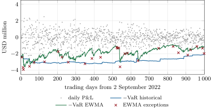
Recomputing each model every day from 2 September 2022 to 23 September 2026, on the same book revalued at each day’s levels, against the next day’s P&L: historical simulation has 10 exceptions in 1 000 days (Kupiec p-value 1.00) and none in the last 250, green; the EWMA delta-normal model has 28 (Kupiec likelihood ratio 22.0, p-value $3\times10^{-6}$ ) and 8 in the last 250, yellow with a 0.75 increase; filtered historical simulation has 8 and 3, green (Figure 21.3). None fails the independence test at 5%.

Figure 21.3. Four years of the book’s daily P&L against the negative of the previous day’s 99% VaR from historical simulation and from the EWMA delta-normal model; crosses mark the EWMA model’s exceptions. The EWMA line reacts to volatility quickly but runs too close to zero for fat-tailed days. Data: US Treasury, ECB; the chapter’s tutorial.

As of September 2026 — VaR and ES in the rules

RiskMetrics was launched by J.P. Morgan in October 1994 (fourth edition of its technical document, with Reuters, December 1996), with decay factors of 0.94 for daily and 0.97 for monthly horizons. The Basel Committee’s 1996 backtesting framework set the traffic light for 99% VaR over 250 days. Its 2019 market-risk standard replaced VaR by expected shortfall at 97.5% on a ten-day base horizon, with desk-level backtests at 97.5% and 99%: more than 12 exceptions at 99% or 30 at 97.5% in twelve months send a desk to the standardised approach.

21.5 Risk contributions

Parametric VaR is homogeneous of degree one in the positions, so Euler allocation (chapter 20) splits it into contributions that add up: $c_i = z_\alpha\delta_i(\Sigma\delta)_i/\sigma$ .

Example 21.18 (Where the risk sits)

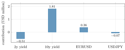
Of the EWMA VaR of USD 1.58 million, the ten-year bond contributes 114%, EURUSD 23%, the two-year short $-32\%$ and the yen short $-5\%$ (Figure 21.4): the two-year hedges part of the ten-year’s rate risk, and the negative contributions mark hedges.

**Figure 21.4.** Euler contributions of each risk factor to the book’s EWMA 99% VaR. They add up to the VaR; negative contributions come from positions that hedge the rest. Data: the chapter’s tutorial.

21.6 Tutorial: VaR on public data

Goal. Compute historical, parametric, Monte Carlo and filtered VaR and ES of the book on Treasury and ECB data, backtest them over four years, and allocate the VaR. End state: the numbers of Examples 21.9, 21.17 and 21.18 and the five charts.

Data: data() joins the par yields and the ECB rates; changes() gives the factor moves.
Measures: measures() runs every method on the last 500 days.
Backtest: backtest() rolls the models over 1 000 days.
Charts: fig_rc_var.py.

What to change next. Use $\lambda = 0.97$ ; drop the straddle and compare delta and full revaluation; shorten the window to 250 days and watch the historical VaR react.

21.7 Build: the VaR model

Purpose. The firm’s market-risk measures and their tests, used by the stress, capital and risk-engine chapters that follow.

Interface. hs_var_es(pnl, alpha); ewma_cov, ewma_vol_path, fhs_scenarios; parametric_var_es, euler_var; mc_var_es(revalue, cov, alpha); delta_gamma; kupiec, christoffersen, traffic_light; sqrt_time.

Rules. Losses positive; historical VaR is the $\lceil(1-\alpha)n\rceil$ -th largest loss and ES the average of that many; EWMA weights normalised; traffic light for 250 days.

Acceptance tests. code/firm/varmodel/tests/: VaR and ES of a known sample; Monte Carlo against parametric for a linear book; Euler contributions add up; normal ES at 97.5% near VaR at 99%; Kupiec zero at the expected count; traffic-light boundaries; Christoffersen detects clustering; filtered scenarios carry today’s volatility.

Stretch. Extreme-value tails; GARCH filtering; ES backtests; stressed calibration; component ES.

Sources and further reading

J.P. Morgan/Reuters, RiskMetrics — Technical Document, 4th ed., 1996.
P. Artzner, F. Delbaen, J.-M. Eber and D. Heath, “Coherent measures of risk”, Mathematical Finance 9(3), 1999, 203–228.
P. Kupiec, “Techniques for verifying the accuracy of risk measurement models”, Journal of Derivatives 3(2), 1995, 73–84.
P. Christoffersen, “Evaluating interval forecasts”, International Economic Review 39(4), 1998.
Basel Committee on Banking Supervision, backtesting framework (1996); Minimum capital requirements for market risk (2019).

21.8 Exercises

Exercise 21.1 ★

With 500 historical days, which loss is the 99% VaR and which losses make up the 97.5% ES?

Solution

Solution of Exercise 21.1.

$k = \lceil0.01\times500\rceil = 5$ : the fifth-largest loss is the VaR. For ES at 97.5%, $\lceil0.025\times500\rceil = 13$ : the average of the thirteen largest losses.

Exercise 21.2 ★

Scale the EWMA one-day VaR to ten days with the square-root-of-time rule. When is the rule wrong?

Solution

Solution of Exercise 21.2.

$1.58\text{ million}\times\sqrt{10} = \text{USD}~5.01$ million. The rule fails when changes are autocorrelated (trends, mean reversion), when volatility changes over the ten days, when the positions are not held (dynamic hedging) and for non-linear books, whose ten-day P&L is not ten one-day P&Ls.

Exercise 21.3 ★

A model has 7 exceptions in 250 days. Give the zone and the multiplication factor.

Solution

Solution of Exercise 21.3.

Yellow, with an increase of 0.65: a multiplication factor of 3.65.

Exercise 21.4 ★★

Verify the numbers of Example 21.13.

Solution

Solution of Exercise 21.4.

Alone: $\P(L>0) = 0.9\% < 1\%$ , so VaR is 0; the worst 1% contains the 0.9% default (100) and 0.1% of zeros, ES $= 0.9\times100/1 = 90$ . Together: $\P(L>0) = 1-0.991^2 = 1.79\% > 1\%$ while $\P(L>100) = 0.0081\% < 1\%$ , so VaR is 100; the worst 1% holds 0.0081% of 200 and 0.9919% of 100, ES $= 100.8$ .

Exercise 21.5 ★★

Why does the short straddle make delta-only VaR too low?

Solution

Solution of Exercise 21.5.

A short straddle has negative gamma: it loses $\tfrac12\Gamma(\Delta S)^2$ on moves in either direction. A delta-only revaluation misses that loss, which is largest in exactly the tail scenarios that set VaR; historical VaR is USD 1.91 million with delta alone and 2.10 with the gamma term.

Exercise 21.6 ★★

Why did the EWMA model fail the Kupiec test while tracking volatility well?

Solution

Solution of Exercise 21.6.

Tracking volatility sets the scale right on average, but the normal distribution puts too little probability in the tails: at the 99% quantile, fat-tailed moves exceed $2.33\hat\sigma$ more often than 1% of the time. Exceptions come from the shape, not the level.

Exercise 21.7 ★★★

Coding. Compute the Kupiec statistic and p-value for 28 exceptions in 1 000 days at 1%.

Solution

Solution of Exercise 21.7.

kupiec(1000, 28, 0.01) gives a likelihood ratio of 22.0 and a p-value of $3\times10^{-6}$ : the model is rejected.

Exercise 21.8 ★★★

Find the flaw. “Our historical VaR had no exception in the last 250 days, so it is too conservative and we should switch to the lower EWMA number.”

Solution

Solution of Exercise 21.8.

Zero exceptions in 250 days happens with probability 8.1% for a correct model: weak evidence of conservatism. Over four years the historical model had exactly 1% exceptions, while the EWMA model, though lower, failed the Kupiec test with 2.8%. Lower is not better.

21.9 Problem: The Quarter-Past-Four Report

Problem 21.1

Weekend problem — one number, and what it costs

The book of Example 21.3 is a desk whose capital is set by its EWMA delta-normal model under the 1996 framework: three (plus the backtesting increase) times the ten-day 99% VaR, scaled from one day.

Part I — The number.

Give the desk’s one-day 99% VaR and 97.5% ES from the EWMA model and from historical simulation.
Which risk factor dominates, and by how much?
Give the ten-day VaR.
Why is the ES barely above the VaR in the EWMA model?
Which number would you report to the board, and why?

Part II — The backtest.

Give the exceptions over the last 250 days and the zone.
Give the multiplication factor.
Give the capital with and without the increase.
How many exceptions did historical simulation have in the same year?
Would filtered historical simulation change the capital?

Part III — The model.

Why does a normal model with fast volatility still have too many exceptions?
What would the 2019 standard require instead of this VaR?
How would the desk fare under its 12- and 30-exception rule?
What does the independence test add?
Which model would you propose, and what would it cost in capital?

Part IV — Judgement.

Why is the lowest VaR not the best model?
Can a desk game a VaR limit? How?
What should the quarter-past-four report contain besides VaR?
State the named result: the desk’s 99% VaR and 97.5% ES, its exceptions over 250 days and the capital multiplier they imply.
In one sentence: what does VaR measure and what does it not?

Solution

Solution of Problem 21.1.

1. EWMA: VaR USD 1.58 million, ES 1.59 million; historical: 2.10 and 2.34 million. 2. The ten-year yield: 114% of the EWMA VaR, partly offset by the two-year short. 3. USD 5.01 million. 4. Under normality ES at 97.5% is 2.338 standard deviations and VaR at 99% 2.326. 5. The historical figures, or both with an explanation: the board needs the fat-tailed number and its uncertainty, not the lowest one. 6. 8 exceptions, yellow zone. 7. $3+0.75 = 3.75$ . 8. USD 15.02 million at 3, 18.78 million at 3.75, taking today’s ten-day VaR for the sixty-day average. 9. None. 10. Yes: with 3 exceptions it would be green with no increase, although its VaR is higher (USD 2.09 million); the capital comparison depends on the level against the multiplier. 11. Its shape is wrong: the normal tail is too thin for these factors. 12. Expected shortfall at 97.5% on a ten-day base horizon scaled by liquidity horizons, with desk-level backtesting and the P&L attribution test (chapter 23). 13. 8 exceptions at 99% is within the 12 allowed; the 97.5% count would also have to stay under 30. 14. Whether exceptions cluster: a model can have the right count but fail in bursts, which is worse for capital adequacy. 15. Filtered historical simulation: fat tails and fast volatility, green over four years; its VaR is higher, but without a multiplier increase its capital is comparable. 16. A model’s job is to be right about the tail; a low number that is exceeded too often understates capital and misleads limits. 17. Yes: by concentrating risk in positions whose losses sit beyond the quantile (short options, credit), by trading on stale windows, or by exploiting factors the model omits. 18. ES, stress results, the largest contributions, concentration and liquidity, limit usage, and backtesting results. 19. Named result: the quarter-past-four report: a 99% VaR of USD 1.58 million and a 97.5% ES of 1.59 million, 8 exceptions in 250 days, and a multiplier of 3.75. 20. A loss exceeded with a given small probability under recent conditions; not how large losses are beyond it, nor what happens when conditions change.

21.10 Interview questions

Interview question 21.1 ★ risk, trader

Define VaR and ES. Why did regulators move from one to the other?

Solution

Solution of Interview question 21.1.

VaR: the loss quantile at a confidence level over a horizon. ES: the average loss beyond that quantile. ES sees the tail’s size and is coherent (subadditive), so it cannot be improved by hiding risk beyond the quantile or penalise diversification.

What the interviewer is looking for: the definitions and the tail and coherence arguments.

Interview question 21.2 ★★ risk

Compare historical simulation, parametric and Monte Carlo VaR.

Solution

Solution of Interview question 21.2.

Historical: real joint moves and fat tails, full revaluation, but slow to react and limited to the window. Parametric: fast and analytic, linear and normal. Monte Carlo: any distribution and full revaluation, but model-dependent and costly.

What the interviewer is looking for: trade-offs of assumptions, speed and nonlinearity.

Interview question 21.3 ★★ researcher, risk

Show that VaR is not subadditive with an example.

Solution

Solution of Interview question 21.3.

Two independent bonds each defaulting with probability 0.9%: each has 99% VaR 0, the pair 100.

What the interviewer is looking for: a concrete counterexample.

Interview question 21.4 ★★ risk, bank

How do you backtest a VaR model? What do the Kupiec and Christoffersen tests check?

Solution

Solution of Interview question 21.4.

Count days whose loss exceeds the previous day’s VaR; Kupiec tests whether the frequency matches the level; Christoffersen tests whether exceptions are independent over time; the traffic light maps counts to capital penalties.

What the interviewer is looking for: frequency and independence.

Interview question 21.5 ★★★ developer

A historical VaR on 100 000 trades with full revaluation takes six hours. How do you make it fast?

Solution

Solution of Interview question 21.5.

Revalue by trade type with vectorised or grid pricing, sensitivities for linear trades, cache scenario-independent terms, parallelise by trade and scenario, run incrementally for changed trades, and keep full revaluation for the non-linear tail.

What the interviewer is looking for: grids, sensitivities and parallelism.

Interview question 21.6 ★★★ researcher

How would you backtest expected shortfall?

Solution

Solution of Interview question 21.6.

ES is not elicitable alone, but joint VaR–ES tests work: compare realised tail losses with the predicted ES on exception days, or backtest the VaR at several levels (the FRTB uses 97.5% and 99%).

What the interviewer is looking for: tail-loss comparisons and multi-level VaR tests.

Terms defined in this chapter

See all 2333 terms in the glossary