Rates, Credit, XVA and Risk · Rates, credit & risk
8Forward-Rate and Market Models
For twenty years before 1997, traders priced caps with Black’s formula applied to each forward rate as if it were a stock, knowing that the formula came from no consistent model of the curve: the lognormal forward of one caplet and the lognormal forward of the next could not both be lognormal under the same measure, and short-rate models priced caps with other formulas. In 1997 three papers, by Brace, Gatarek and Musiela, by Jamshidian, and by Miltersen, Sandmann and Sondermann, showed that the traders’ formula was exactly right in a model in which every forward rate is lognormal under the measure of its own payment date, and that one such model could hold all forwards at once. The market model, as it came to be called, calibrates to caplets by construction, needs Monte Carlo for almost everything else, and makes visible a parameter the short-rate models hid: the correlation between forward rates. This chapter derives the general framework it belongs to, builds and simulates it, and shows two correlations that fit the same caplets and price the same swaption 22% apart.
8.1 The Heath–Jarrow–Morton framework and its drift
Definition 8.1 (Heath–Jarrow–Morton framework)
The Heath–Jarrow–Morton framework (1992) models the whole instantaneous forward curve: for each maturity , under , starting from today’s curve , with volatilities chosen freely (vectors for several factors).
Definition 8.2 (HJM drift condition)
The HJM drift condition is the restriction that absence of arbitrage imposes on the drift once the volatilities are chosen:
Proposition 8.3 (Why the drift is fixed)
Bond prices discounted by the bank account are -martingales if and only if the drift condition holds.
Proof. with . By Itô’s formula the drift of is ; it vanishes for all iff , and differentiating in gives the condition. ∎
Example 8.4 (Hull–White is an HJM model)
Chapter 7’s model has : its drift is , 4.1 basis points a year for the ten-year forward with basis points and . Volatilities of this exponential form are exactly those for which the forward curve is driven by a single Markov state; a general makes the short rate path-dependent and the model can only be simulated.
8.2 The market model
The instantaneous forward is not traded. The market model takes the forwards that are: for the accrual periods of a tenor structure.
Definition 8.5 (LIBOR market model)
The LIBOR market model (or lognormal forward market model) makes each forward rate lognormal with a deterministic volatility under the forward measure of its payment date: , with . Its name comes from the interbank index it was built for; the dynamics serve any tenor structure of forward-looking rates, and chapter 10 extends them to overnight-rate compounding.
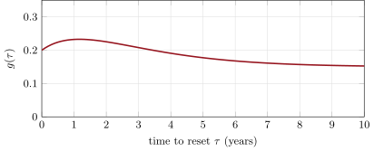
Each caplet is then priced exactly by Black’s formula with volatility , which is what makes the model calibrate to caps by construction. A common volatility form is Rebonato’s
a hump in the time to reset scaled by a constant per forward (Figure 8.1); the are solved so that every caplet reprices.
8.3 Drifts under the spot and terminal measures
To simulate all forwards together they must share one measure, and under any single measure all but one of them acquire a drift.
Definition 8.6 (Spot measure, terminal measure)
The spot measure of a tenor structure has as numeraire the discretely rebalanced bank account , which holds the bond maturing at the next reset date and rolls into the next one at each reset. The terminal measure is the forward measure of the last payment date , with numeraire .
Proposition 8.7 (Market-model drifts)
Under the spot measure, for a forward alive at ,
and under the terminal measure the drift is .
Partial proof. Change numeraire one period at a time: the density of with respect to is proportional to , whose volatility is ; by Girsanov’s theorem (One Quant Book 4, chapter 5) each change adds the covariance of with that density to the drift. Summing from the numeraire’s bond to ’s own payment date gives both formulas. ∎
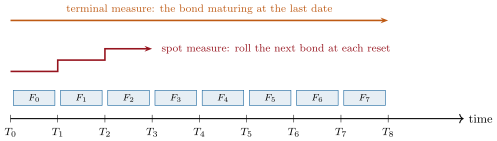
Simulation steps with the drift evaluated at the start of the step (Euler) and again at the predicted end, averaging the two (predictor–corrector): the drift depends on the forwards themselves, and the correction keeps the simulated caplets on their Black prices at coarse steps.
def spot_drift(fv: np.ndarray, sig: np.ndarray, rho: np.ndarray, nxt: int, delta: float) -> np.ndarray:
    """Drift of each ln F_k under the spot measure (Ito term excluded):
    sigma_k sum_{j=nxt}^{k} delta rho_kj sigma_j F_j / (1 + delta F_j)."""
    x = delta * sig * fv / (1 + delta * fv)                        # paths x n
    mu = np.zeros_like(fv)
    for k in range(nxt, fv.shape[1]):
        mu[:, k] = sig[k] * (x[:, nxt:k + 1] @ rho[k, nxt:k + 1])
    return mu


def simulate(m: LMM, horizon: int, paths: int, sub: int = 4, seed: int = 7):
    """Forwards on the reset grid under the spot measure: returns (F at each reset date 0..horizon,
    numeraire B_d at each reset date). F[t][p, k] is F_k at T_t on path p."""
    rng = np.random.default_rng(seed)
    n, dt, rho = m.n, 1.0 / sub, m.corr()
    chol = np.linalg.cholesky(rho)
    logf = np.tile(np.log(m.f0), (paths, 1))
    out, numer = [np.exp(logf).copy()], [np.ones(paths)]
    bd = np.ones(paths)
    for step in range(horizon * sub):
        t = step * dt
        nxt = int(math.floor(t + 1e-12)) + 1                      # first forward still alive after t
        z = rng.standard_normal((paths, n)) @ chol.T
        sig = np.array([m.vol(k, t) for k in range(n)])
        mu0 = spot_drift(np.exp(logf), sig, rho, nxt, m.delta)          # predictor
        pred = logf + (mu0 - 0.5 * sig**2) * dt + sig * math.sqrt(dt) * z
        mu1 = spot_drift(np.exp(pred), sig, rho, nxt, m.delta)          # corrector
        alive = np.arange(n) >= nxt
logf = np.where(alive, logf + (0.5 * (mu0 + mu1) - 0.5 * sig**2) * dt + sig * math.sqrt(dt) * z, logf)Example 8.8 (Caplets come back)
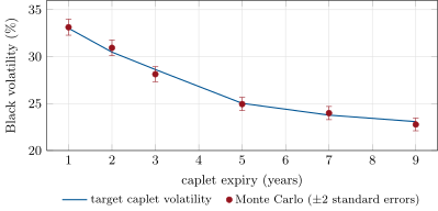
Ten annual forwards from chapter 2’s euro OIS curve (1.98% for the first year rising to 3.03% for the tenth), caplet volatilities of 70 basis points normal converted to Black (33.0% at one year down to 23.1% at nine), Rebonato’s function with the parameters of Figure 8.1 and correlation : 20 000 paths under the spot measure, four steps a year, reprice the at-the-money caplets to within two standard errors (Figure 8.3).
8.4 Calibrating to caps and swaptions: Rebonato’s formula
A swap rate is a weighted average of forwards, with , so its volatility follows from theirs and their correlations.
Definition 8.9 (Swap market model)
A swap market model makes chosen swap rates lognormal under their own annuity measures, so that swaptions are priced by Black’s formula. It cannot hold together with a lognormal market model of the forwards: a weighted sum of lognormals is not lognormal. Desks use one and approximate the other.
Definition 8.10 (Rebonato’s formula)
Rebonato’s formula approximates the Black volatility of the swaption expiring at on in the market model by freezing the weights and the forwards at today’s values:
def rebonato_vol(m: LMM, a: int, b: int) -> float:
    """Black volatility of the swaption expiring at T_a on the swap [T_a, T_b], by Rebonato's formula."""
    s, _, w = m.swap(a, b)
    rho = m.corr()
    tot = 0.0
    for i in range(a, b):
        for j in range(a, b):
            tot += w[i - a] * w[j - a] * m.f0[i] * m.f0[j] * rho[i, j] * m.integrated_cov(i, j, float(a))
return math.sqrt(tot / (s * s * a))8.5 Correlation and factor reduction
Definition 8.11 (Forward-rate correlation)
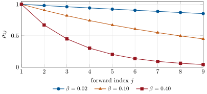
The forward-rate correlation of a market model is the instantaneous correlation of the Brownian motions driving and . It is usually parametrised, for example , and reduced to two or three factors by keeping the leading eigenvectors of the matrix (the principal components of chapter 3), which speeds simulation and removes noise.
Caplets do not depend on correlation; swaptions do, since a swap rate averages several forwards and averaging decorrelated rates reduces volatility. A market model calibrated to caplets alone therefore leaves its swaption prices to an assumption.
Example 8.12 (Same caplets, different swaptions)
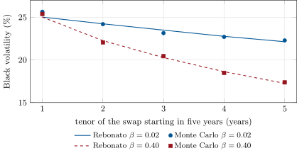
Calibrate the model to the same caplets with (forwards nearly perfectly correlated) and with (the one-year and nine-year forwards correlated at 0.04). The swaption expiring in five years into one year is priced at 25.0% of Black volatility by both (it is one forward); into five years, at 22.1% and 17.3% (Figure 8.5). On EUR 100 million, at the money (forward 2.933%, annuity 4.102), that is EUR 2.35 million against 1.84 million: 22% apart for the same caplets. Monte Carlo confirms Rebonato’s formula to within its standard errors.
Remark 8.13 (Calibrating the correlation)
Desks calibrate the market model jointly: the to caplets or co-terminal swaptions, the volatility shape and the correlation to the swaption matrix, often by fitting (or a two-parameter form) to historical forward-rate correlations and letting the swaptions fix the rest. A product depending on the correlation of rates that no liquid instrument pins down carries a reserve for it (Chapter 27).
8.6 Tutorial: a market model on the euro curve
Goal. Calibrate a market model to caplets, simulate it, and measure how correlation moves swaptions. End state: Figures 8.3 and 8.5.
- Forwards and targets:
F0from chapter 2’s €STR curve, caplet Black volatilities from 70 basis points normal. - Calibrate:
calibrate_to_caplets(F0, vols, abcd, beta)solves the . - Simulate:
mc_capletandmc_swaptionunder the spot measure;caplet_check(). - Correlation:
swaption_table()for and ;fig_rc_lmm.pywrites the charts.
What to change next. Simulate under the terminal measure and compare standard errors; reduce the correlation matrix to two factors and measure the change in the five-into-five volatility.
8.7 Build: a market-model engine
Purpose. The benchmark model for products that depend on several rates at several dates: Bermudans (chapter 9), CMS spread options (chapter 6), and the validation of chapter 7’s one-factor model.
Interface. LMM(f0, phi, abcd, beta) with vol, corr, integrated_cov, discount_factors, swap; calibrate_to_caplets; rebonato_vol; simulate, mc_caplet, mc_swaption; hjm_drift_gaussian.
Rules. Annual tenor structure, lognormal forwards, spot measure with predictor–corrector steps; fixed seeds; numpy only.
Acceptance tests. code/firm/lmm/tests/: the calibrated integrated variances match the caplet targets and Rebonato’s formula for a one-period swaption returns the caplet volatility; Monte Carlo reprices a caplet within three standard errors; a deep in-the-money swaption is the forward swap; lower correlation lowers swaption volatility; the Hull–White HJM drift has its closed form.
Stretch. Shifted or normal forwards for low rates; a stochastic-volatility market model; calibration of to the swaption matrix.
Sources and further reading
- D. Heath, R. Jarrow and A. Morton, “Bond pricing and the term structure of interest rates”, Econometrica 60(1), 1992.
- A. Brace, D. Gatarek and M. Musiela, “The market model of interest rate dynamics”, Mathematical Finance 7, 1997; F. Jamshidian, “LIBOR and swap market models and measures”, Finance and Stochastics 1, 1997; K. Miltersen, K. Sandmann and D. Sondermann, Journal of Finance 52(1), 1997.
- R. Rebonato, Modern Pricing of Interest-Rate Derivatives: The LIBOR Market Model and Beyond, Princeton University Press, 2002.
8.8 Exercises
Exercise 8.1 ★
In an HJM model with constant, what is the drift of ? Which short-rate model is it?
Solution
Solution of Exercise 8.1.
. It is the Hull–White model with no mean reversion (), known as the Ho–Lee model: every forward moves by the same normal shock.
Exercise 8.2 ★
Why is each caplet priced exactly by Black’s formula in the market model, but not each swaption?
Solution
Solution of Exercise 8.2.
Each forward is a martingale under its own payment measure with a deterministic volatility, so it is lognormal there and its caplet is Black’s formula. A swap rate is a weighted sum of several forwards with stochastic weights; it is not lognormal under its annuity measure, so Black is only an approximation.
Exercise 8.3 ★
With , what is the correlation between the first and the ninth annual forwards? With ?
Solution
Solution of Exercise 8.3.
; with , .
Exercise 8.4 ★★
Under the spot measure, write the drift of at in a model with annual forwards. Which forwards appear?
Solution
Solution of Exercise 8.4.
At the next reset is , so : ; and appear ( has already reset).
Exercise 8.5 ★★
Two forwards of 3% with Black volatility 20% each, weights 0.5 each and correlation . With Rebonato’s formula, what is the swap-rate volatility for and ?
Solution
Solution of Exercise 8.5.
: 20.00% for , 17.32% for .
Exercise 8.6 ★★
Read Figure 8.5: why do both models agree on the five-into-one swaption?
Solution
Solution of Exercise 8.6.
A one-year swap starting in five years is a single annual forward, : its swaption is a caplet, priced by its own volatility, which both models calibrate to the same target; correlation needs at least two forwards to matter.
Exercise 8.7 ★★★
Coding. Price the five-into-five at-the-money payer on EUR 100 million under both correlations with Rebonato’s formula, and give the difference.
Solution
Solution of Exercise 8.7.
EUR 2 351 823 with , EUR 1 840 368 with : a difference of EUR 511 456.
Exercise 8.8 ★★★
Find the flaw. “We simulate the market model under the spot measure with each forward’s drift set to zero, because each forward is a martingale.”
Solution
Solution of Exercise 8.8.
Each forward is a martingale only under its own payment measure; under a common simulation measure all but one have a drift (Proposition 8.7). With zero drifts the simulation misprices every caplet except the one whose measure is the numeraire’s, by an error growing with maturity and volatility, and the discounting by the spot account is inconsistent with the forwards.
8.9 Problem: The Correlation You Cannot See
Problem 8.1
Weekend problem — a market model calibrated to caplets
A desk runs a ten-forward annual market model on the euro OIS curve, calibrated every morning to caplets at 70 basis points of normal volatility. A client asks for the five-into-five at-the-money payer swaption on EUR 100 million. The desk’s correlation parameter has never been calibrated.
Part I — What the caplets fix.
- Give the forward swap rate and the annuity.
- Which parameters do the caplets determine, and which not?
- Give the caplet Black volatilities at one and nine years.
- Why is the five-into-one swaption the same under any correlation?
- What else is left free by the calibration?
Part II — Two correlations.
- Give the five-into-five volatility with and with .
- Give the two premiums.
- Give the relative difference.
- How well does Rebonato’s formula agree with Monte Carlo here?
- Which correlation would you expect from historical data, and why?
Part III — Fixing it.
- Which instruments would pin down the correlation?
- If the market quotes the five-into-five at 20%, what does it imply (bracket it)?
- After calibrating to it, what would still be unpinned?
- How does the choice of change the desk’s hedges?
- Why is a one-factor Hull–White model equivalent to ?
Part IV — Judgement.
- Which price would you quote, and what reserve would you hold?
- How would you monitor the parameter over time?
- What should the model documentation say about ?
- State the named result: the five-into-five premiums under the two correlations and their difference.
- In one sentence: what does a swaption know that a caplet does not?
Solution
Solution of Problem 8.1.
1. 2.933% and 4.102. 2. The integrated variance of each forward up to its reset (the given the volatility shape); not the correlation, and not how each forward’s variance is spread in time beyond what the chosen shape imposes. 3. 33.0% and 23.1%. 4. It depends on a single forward, . 5. The shape parameters , which move variance between early and late times and so change swaptions of different expiries and forward volatilities. 6. 22.1% and 17.3%. 7. EUR 2.35 million and 1.84 million. 8. 22%. 9. Within about two standard errors (under 0.9 volatility points on every five-year-expiry swaption). 10. Something like chapter 6’s Treasury estimate of 0.77 between two- and ten-year changes: forward rates a few years apart are highly but not perfectly correlated, which points to between the two extremes. 11. Swaptions on longer swaps (the swaption matrix), CMS spread options where traded. 12. About 0.16: with Rebonato’s formula gives 20%. 13. The whole shape of the correlation matrix beyond one parameter, the time dependence of correlation, and anything depending on joint moves at other expiries. 14. It changes the swaption vegas’ split across forwards and the hedge ratios between caps and swaptions: a book hedged with caps against swaptions carries correlation risk. 15. One factor moves all rates together: perfect correlation, the limit . 16. The price at a calibrated to the quoted swaption matrix, with a reserve covering a plausible range of correlation (here the difference between values bracketing history and implied levels). 17. Track the calibrated and historical correlations daily, alert on jumps, and report the P&L from re-marking separately. 18. How it is chosen, what instruments it is calibrated to, its range, the products sensitive to it and the reserve held. 19. Named result: the correlation you cannot see: with the same caplets, the five-into-five payer is worth EUR 2.35 million with and EUR 1.84 million with , 22% (EUR 511 456) apart. 20. How rates of different maturities move together.
8.10 Interview questions
Interview question 8.1 ★ researcher
State the HJM drift condition and explain where it comes from.
Solution
Solution of Interview question 8.1.
under the risk-neutral measure. It comes from requiring every discounted bond price to be a martingale: the bond’s log-price drift, , must equal for every maturity; differentiate in .
What the interviewer is looking for: no arbitrage on bonds, and the derivation in two lines.
Interview question 8.2 ★★ researcher, developer
How do you simulate a LIBOR market model, and why is there a drift?
Solution
Solution of Interview question 8.2.
Choose a measure (spot or terminal), write each forward’s drift from the covariance with the numeraire change, and step with correlated normals, a predictor–corrector drift and the numeraire rolled at resets. The drift is there because each forward is a martingale only under its own payment measure.
What the interviewer is looking for: common measure, drift from numeraire change, log stepping.
Interview question 8.3 ★★ researcher, trader
Why can caplets and swaptions not both be exactly lognormal?
Solution
Solution of Interview question 8.3.
A swap rate is an average of forwards with random weights; if forwards are lognormal under their measures, a swap rate is not lognormal under its annuity measure, and vice versa. One of the two sets is priced by Black only approximately.
What the interviewer is looking for: sums of lognormals are not lognormal.
Interview question 8.4 ★★ trader
You calibrate a market model to caplets only. What is wrong with your swaption prices?
Solution
Solution of Interview question 8.4.
Caplets fix each forward’s variance but not their correlation, which drives swaption volatilities: the swaption prices are set by an arbitrary correlation assumption, here up to 22% apart. Calibrate to swaptions too.
What the interviewer is looking for: correlation as the missing input.
Interview question 8.5 ★★★ researcher, risk
Compare Hull–White and the market model for pricing a ten-year Bermudan.
Solution
Solution of Interview question 8.5.
Hull–White: fast (trees), exact co-terminal fit with , one factor so perfectly correlated exercises, which understates the switch value. Market model: flexible correlation and smile extensions, calibrated to caplets and swaptions, but needs regression Monte Carlo for early exercise and is slower and noisier. Use Hull–White in production, the market model as benchmark.
What the interviewer is looking for: speed versus correlation, and a production/benchmark split.
Interview question 8.6 ★★★ developer
Your simulated caplet prices drift away from Black as you use coarser time steps. What is happening, and what do you change?
Solution
Solution of Interview question 8.6.
Discretisation bias of the drift: an Euler drift evaluated at the start of long steps is wrong because it depends on forwards that move within the step. Use a predictor–corrector, finer steps near resets, or a measure that puts the numeraire’s drift-free forward where it matters; check caplets against Black at each step size.
What the interviewer is looking for: drift discretisation and a convergence check.