Rates, Credit, XVA and Risk · Rates, credit & risk
16Commodity and Energy Derivatives
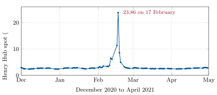
In the second week of February 2021 a cold snap froze gas wells across Texas and the southern plains. Spot gas at the Waha hub in West Texas reached 206.19 dollars per million British thermal units on 16 February; at one Oklahoma hub the average price on 17 February was 1 192 dollars, against under 3 dollars in the first week of the month, according to the US Energy Information Administration. Henry Hub, the benchmark, went from 2.88 dollars on 1 February to 23.86 on the 17th and back under 3 by the 23rd. For a week, the value of gas in the ground depended on how fast it could be taken out: an owner of a salt cavern that can empty in days could sell at the peak, one with a slow reservoir could not. This chapter values that flexibility. One Quant Book 3 described the forward curves, storage economics and structured contracts of commodity markets; here they get models: a forward curve that moves in two factors, options on the spread between two prices, and the valuation of storage and swing rights by optimisation under uncertainty.
16.1 Factor models of the forward curve
A commodity has a forward curve rather than a price: each delivery month trades, with seasonal shape and a convenience yield (One Quant Book 3, chapter 10). A model must move the whole curve, and it must let short-dated contracts move more than long-dated ones.
Definition 16.1 (Schwartz–Smith model)
The Schwartz–Smith model writes the log spot price as the sum of a short-term deviation , an Ornstein–Uhlenbeck process reverting to zero at speed with volatility , and a long-term level , a Brownian motion with volatility , the two correlated by . Its forward curve moves as
so that with the variance. Seasonality sits in the initial curve , which the model fits exactly.
Both factors are Gaussian and simulated exactly, and each forward is lognormal: an option on the forward expiring at is priced by Black’s formula with the implied volatility .
Example 16.2 (Calibration)
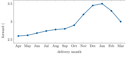
An illustrative Henry Hub-like curve runs from 2.60 dollars for April to 3.50 for January. Options expiring half a month before each delivery are quoted at implied volatilities falling from 62.0% (May) to 43.0% (March), synthetic. With fixed, a Levenberg–Marquardt fit gives , and .
16.2 The Samuelson effect and forward volatility
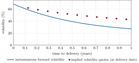
In the model the instantaneous volatility of a forward with time to delivery is
68.7% at delivery, 27.2% one year out and 20.0% five years out for the calibrated parameters. This is the Samuelson effect of One Quant Book 3 as a model property: shocks to supply and demand move near contracts, which the short-term factor carries, while far contracts move only with the long-term level (Figure 16.1). The correlation between two contracts falls with the distance between their deliveries, which is what makes spread options worth something.
16.3 Spread options
Definition 16.3 (Spread option)
A spread option pays on the difference between two prices: two delivery months of one commodity (a calendar spread), a product and its input (a crack or spark spread), or one commodity at two places.
With and lognormal prices the option is an exchange option, priced exactly by Margrabe’s formula with the volatility of the ratio, . With the difference is not lognormal and there is no closed form.
Definition 16.4 (Kirk’s approximation)
Kirk’s approximation prices a spread call by treating as lognormal with volatility and applying Margrabe’s formula:
def kirk(F1: float, F2: float, K: float, T: float, s1: float, s2: float, rho: float, df: float = 1.0) -> float:
    """Kirk's approximation to a call on F1 - F2 - K: F2 + K treated as lognormal with vol s2 F2 / (F2 + K)."""
    b = F2 / (F2 + K)
    s = math.sqrt(s1 * s1 - 2 * rho * s1 * s2 * b + (s2 * b) ** 2)
    d1 = (math.log(F1 / (F2 + K)) + 0.5 * s * s * T) / (s * math.sqrt(T))
return df * (F1 * ND.cdf(d1) - (F2 + K) * ND.cdf(d1 - s * math.sqrt(T)))Example 16.5 (A calendar spread)
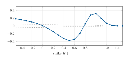
A call on the January forward (3.50) minus the July forward (2.74), strike 0.50, expiring at July delivery: the model gives volatilities of 34.8% and 58.1% to that date and a correlation of 0.970. Kirk’s approximation prices it at 29.41 cents per MMBtu against 29.78 by Monte Carlo (standard error 0.01), an error of 0.38 cent; at zero strike both give about 75.8 cents, Margrabe’s value. The error is largest near the money, where the approximation of the sum’s distribution matters most (Figure 16.2).
16.4 Storage valuation
A storage facility buys gas when it is cheap, holds it and sells it when it is dear, within limits on capacity and on injection and withdrawal rates, and at a cost per unit moved. Its owner holds a portfolio of calendar spread options linked by the inventory.
Definition 16.6 (Intrinsic storage value)
The intrinsic storage value of a facility is the value of the best injection and withdrawal schedule on today’s forward curve, locked in by trading the forwards: a deterministic optimisation.
Definition 16.7 (Extrinsic value, rolling intrinsic)
The extrinsic value of a facility is its value above the intrinsic, from the right to change the schedule as prices move. The rolling intrinsic strategy captures part of it: re-optimise the schedule on each new forward curve and re-hedge the difference, never losing the intrinsic already locked in.
Method 16.8 (Storage by least-squares Monte Carlo)
Simulate spot prices for each period. Work backwards from the last period with the value of each end inventory known on each path. At each period and for each inventory level reachable after the action, regress the next period’s realised value on , and to estimate the continuation value; choose, path by path, the action that maximises cash now plus estimated continuation, and carry back the realised value of that choice. The value is the average at the starting inventory.
def lsm(fac: Facility, spot: np.ndarray, dfs: list[float], degree: int = 2) -> float:
    """Least-squares Monte Carlo value of the facility on simulated spot (paths x periods)."""
    npaths, n = spot.shape
    cap = fac.capacity
    V = np.full((npaths, cap + 1), -1e18)
    V[:, fac.end if fac.end >= 0 else slice(None)] = 0.0
    for m in range(n - 1, -1, -1):
        S = spot[:, m]
        X = np.column_stack([S ** d for d in range(degree + 1)])
        cont = np.empty_like(V)
        for j in range(cap + 1):
            if V[0, j] <= -1e17 and (V[:, j] <= -1e17).all():
                cont[:, j] = -1e18
            else:
                beta, *_ = np.linalg.lstsq(X, V[:, j], rcond=None)
                cont[:, j] = X @ beta
        W = np.full_like(V, -1e18)
        for i in range(cap + 1):
            best_est = np.full(npaths, -np.inf)
            chosen = np.zeros(npaths)
            for a in fac.actions(i):
                if (V[:, i + a] <= -1e17).all():
                    continue
                now = dfs[m] * fac.cash(a, S)
                est = now + cont[:, i + a]
                real = now + V[:, i + a]
                better = est > best_est
                best_est = np.where(better, est, best_est)
                chosen = np.where(better, real, chosen)
            W[:, i] = np.where(np.isfinite(best_est), chosen, -1e18)
        V = W
return float(V[:, fac.start].mean())Example 16.9 (A season of storage)
A facility of 1 million MMBtu (ten units) starts and ends the April–March year empty; it can inject two units a month and withdraw four, at 2 cents per MMBtu each way. On the curve of Example 16.2 the intrinsic plan injects two units a month from April to August and withdraws in December, January and February (Figure 16.3); its value is USD 634 447. Rolling intrinsic on 4 000 simulated curves is worth USD 699 550, least-squares Monte Carlo USD 698 182: an extrinsic value of about 10% of the intrinsic at a monthly decision frequency. Daily decisions, which a fast facility can take, add more.
16.5 Swing contracts
A swing contract (One Quant Book 3, chapter 12) is storage without injection: the holder has a number of rights to take gas at a fixed price, limited per period and in total. The same dynamic programme values it, with the inventory counting rights left.
Example 16.10 (A winter swing)
Rights to take up to 200 000 MMBtu a month from November to March, 600 000 in all, at 3.10 dollars: on the forward curve the best plan takes 200 000 in December, January and February, an intrinsic value of 1.84 per unit of 100 000 MMBtu; least-squares Monte Carlo gives 4.37. Ten monthly calls, two a month without the total limit, are worth 6.11, an upper bound: the limit on the total is what makes the swing cheaper than a strip.
As of September 2026 — February 2021
The US Energy Information Administration reported that during the cold snap of February 2021 the Waha hub reached 206.19 dollars per MMBtu on 16 February and SoCal Citygate 144.00 on 12 February, and that Oneok Gas Transportation in Oklahoma averaged 1 192 dollars on 17 February according to NGI data, against 2.91 in the first week of the month; gas production fell because of well freeze-offs. Henry Hub averaged 5.35 dollars over the month, against 2.71 in January.
16.6 Tutorial: storage under a two-factor curve
Goal. Calibrate the two-factor model, price a calendar spread option, and value a storage facility and a swing contract. End state: the numbers of Examples 16.2, 16.5, 16.9 and 16.10 and the four figures.
- Calibrate:
model()fits , , tovol_quotes(). - Spread:
calendar_spread(0.5);kirk_table()by strike. - Storage:
storage()gives intrinsic, rolling intrinsic and least-squares Monte Carlo values. - Swing and storm:
swing(),storm();fig_rc_energy.pywrites the charts.
What to change next. Double the withdrawal rate and see how much extrinsic value the faster facility adds; set to zero and watch the extrinsic value of the storage shrink.
16.7 Build: the energy model
Purpose. The firm’s commodity engine: forward-curve simulation for the exposure and risk engines of Parts III and IV, spread options, and the valuation of physical flexibility.
Interface. TwoFactor(kappa, sigma_s, sigma_l, rho) with var, cov, implied_vol, simulate, forward; calibrate; margrabe, kirk, spread_mc; Facility; intrinsic, lsm, rolling_intrinsic, spot_paths; swing_facility.
Rules. One decision per delivery period; integer inventory units; spot of a period is its forward at delivery; antithetic simulation.
Acceptance tests. code/firm/energymodel/tests/: simulated forwards are martingales with the model’s variance; calibration recovers the parameters; Kirk equals Margrabe at zero strike and is within 1% of Monte Carlo; a flat curve has no intrinsic storage value; without volatility, least-squares Monte Carlo equals intrinsic; rolling intrinsic and least-squares Monte Carlo exceed intrinsic; a swing’s intrinsic is the sum of its best exercises.
Stretch. Daily decisions within the month; ratchets (rates that depend on the inventory); a jump factor for spikes; the spot-forward basis of a physical hub.
Sources and further reading
- E. S. Schwartz, “The stochastic behavior of commodity prices: implications for valuation and hedging”, Journal of Finance 52(3), 1997, 923–973.
- E. Schwartz and J. E. Smith, “Short-term variations and long-term dynamics in commodity prices”, Management Science 46(7), 2000, 893–911.
- A. Boogert and C. de Jong, “Gas storage valuation using a Monte Carlo method”, Journal of Derivatives 15(3), 2008, 81–98.
- E. Kirk, “Correlation in the energy markets”, in R. Jameson (ed.), Managing Energy Price Risk, Risk Publications and Enron, London, 1995, 71–78.
- US Energy Information Administration, Today in Energy, “Cold weather brings near record-high natural gas spot prices”, February 2021; Henry Hub daily spot series.
16.8 Exercises
Exercise 16.1 ★
With the calibrated parameters, what is the instantaneous volatility of a forward one year from delivery, and why is it lower than at delivery?
Solution
Solution of Exercise 16.1.
27.2%, against 68.7% at delivery. The short-term factor’s loading has decayed to : a forward a year out moves mainly with the long-term level, because shocks to today’s supply and demand are expected to fade before it delivers.
Exercise 16.2 ★
Why is the intrinsic value of storage zero on a flat forward curve, and why is the facility still worth something?
Solution
Solution of Exercise 16.2.
Every schedule buys and sells at the same forward price and pays the injection and withdrawal costs, so the best deterministic plan is to do nothing. The facility is still a portfolio of spread options: as prices move, spreads between months open and the owner can exploit them; its value is all extrinsic.
Exercise 16.3 ★
A calendar spread call with strike 0.50 on forwards at 3.50 and 2.74 expires tomorrow. What is it worth?
Solution
Solution of Exercise 16.3.
Its intrinsic value, discounted one day: dollars per MMBtu (0.2600 after a day’s discounting at 4%).
Exercise 16.4 ★★
Why does the correlation between two delivery months matter for a spread option, and in which direction?
Solution
Solution of Exercise 16.4.
The spread’s volatility is (at zero strike): higher correlation means a less volatile spread and a cheaper option. Close delivery months are highly correlated (0.970 for July and January at July’s expiry in the chapter), distant ones less.
Exercise 16.5 ★★
Why can rolling intrinsic never be worth less than intrinsic?
Solution
Solution of Exercise 16.5.
It starts with the intrinsic plan hedged with forwards, and changes the plan only when the new plan, valued on the new curve, is worth more than the old one after re-hedging: each change adds non-negative value locked in by forwards.
Exercise 16.6 ★★
Why is a swing contract worth less than the strip of monthly calls it contains?
Solution
Solution of Exercise 16.6.
The strip gives the right to exercise every monthly call; the swing caps the total, so its holder must choose which months to use, giving up some exercises the strip would take. The strip is an upper bound (6.11 against 4.37 in the chapter).
Exercise 16.7 ★★★
Coding. Compute Kirk’s error at strikes 0 and 0.5 and explain the difference.
Solution
Solution of Exercise 16.7.
At zero strike Kirk’s formula is Margrabe’s, exact for lognormal forwards: the difference from Monte Carlo is 0.007 cent, within the noise. At 0.50 it is cent: the sum is not lognormal, and the approximation of its volatility by is off near the money, where the option is most sensitive to the distribution’s shape.
Exercise 16.8 ★★★
Find the flaw. “Our storage book is valued at intrinsic and fully hedged with forwards, so February 2021 was neither a risk nor an opportunity for us.”
Solution
Solution of Exercise 16.8.
A book hedged at intrinsic is hedged against parallel moves of the forward curve, but it owns options: in February 2021 the right to withdraw fast at spot was worth millions of dollars to a fast facility, and a book that did not use it gave it away. Conversely, a book short flexibility (supply contracts with swing) had a large loss. The intrinsic hedge does not measure either.
16.9 Problem: The Salt Cavern in February 2021
Problem 16.1
Weekend problem — a fast and a slow facility in the cold snap
Two facilities each hold 500 000 MMBtu near Henry Hub on 8 February 2021. The salt cavern can withdraw 100 000 MMBtu a day, the depleted reservoir 10 000. Between 8 and 19 February each may sell on its best days at the daily Henry Hub price, and buys the same volume back at the March 2021 average to restore its plan; moving gas costs 2 cents per MMBtu each way.
Part I — Before the winter.
- Give the intrinsic, rolling intrinsic and least-squares Monte Carlo values of the chapter’s facility.
- What is its extrinsic value, and where does it come from?
- Which parameter of the curve model drives the extrinsic value most?
- Why does a monthly model understate a salt cavern’s extrinsic value?
- How would you hedge the intrinsic value at the start of the season?
Part II — The storm.
- Give Henry Hub on 1 February and at its peak, and the day of the peak.
- Give the March 2021 average used for the buy-back.
- Give the volume the salt cavern sells, on how many days, and its gain.
- Give the same for the depleted reservoir.
- Why is the ratio of the gains not the ratio of the withdrawal rates?
Part III — What a model sees.
- How many standard deviations is the move from 3.76 dollars on 10 February to 23.86 on 17 February (four trading days) under a lognormal model with the chapter’s 69% short-term volatility?
- Which model feature would put such spikes in the simulation?
- Why did the storm raise the value of the facility’s options but not its intrinsic value for the next season?
- Which contracts gained besides storage?
- Who was short that flexibility?
Part IV — Judgement.
- Why do owners of fast storage pay for it when the average year gives little extrinsic value?
- How would you report the storage book’s risk to a risk committee?
- What would you change in the valuation model after February 2021?
- State the named result: the gains of the fast and the slow facility in the storm.
- In one sentence: what is a storage facility worth beyond its seasonal spread?
Solution
Solution of Problem 16.1.
1. USD 634 447, 699 550 and 698 182. 2. About USD 64 000, 10% of the intrinsic: the right to change the schedule as spreads between months move. 3. The short-term volatility , with the mean reversion : they set how much near months move against each other. 4. It lets the facility act once a month on monthly prices; a salt cavern acts daily, on daily prices whose spikes average out in a monthly price. 5. Buy the summer forwards and sell the winter forwards of the intrinsic plan, in the plan’s volumes. 6. 2.88 dollars on 1 February; 23.86 on 17 February. 7. 2.62 dollars. 8. 500 000 MMBtu on five days (11, 12, 16, 17 and 18 February), a gain of USD 4 306 870. 9. 90 000 MMBtu on nine days, a gain of USD 479 057. 10. The cavern runs out of gas after five days and sells only on the best ones; the reservoir sells a little every day, including the days of 3.35 to 3.76 dollars. 11. against : 21 standard deviations, impossible in the model. 12. Jumps (a jump-diffusion or regime-switching spot) or a stochastic volatility that rises with scarcity. 13. The spike lasted a week and left the forward curve for the next season almost unchanged, so the seasonal spread (the intrinsic value) did not move; the options gained because they were exercised in the spike. 14. Swing contracts and other rights to take gas at a fixed price, firm pipeline capacity out of the frozen region, and call options on daily gas. 15. Sellers of those rights: suppliers with swing obligations who had to buy gas at spot to deliver at the contract price, and generators short fuel for their power sales. 16. The value sits in rare, extreme weeks; the average year understates it, and a single event can pay for years of fees. 17. The intrinsic position and its hedges, the extrinsic value and its sensitivity to volatility, the value under historical stress weeks, and the physical limits (rates, ratchets, contracts that could oblige deliveries). 18. Add spikes (jumps or regimes) to the short-term factor, and decide daily. 19. Named result: the salt cavern in February 2021: the fast facility gains USD 4 306 870 on 500 000 MMBtu, the slow one USD 479 057 on 90 000. 20. The options to move gas through time at short notice, which pay most in exactly the weeks no model of the average predicts.
16.10 Interview questions
Interview question 16.1 ★ trader, researcher
What is the Samuelson effect, and how does a two-factor model produce it?
Solution
Solution of Interview question 16.1.
Short-dated forwards are more volatile than long-dated ones. In a two-factor model a mean-reverting short-term factor moves near contracts with loading , fading for distant deliveries, while a long-term factor moves them all.
What the interviewer is looking for: the observation and the mechanism.
Interview question 16.2 ★★ researcher
Price a spread option with a non-zero strike. What approximations exist and when do they fail?
Solution
Solution of Interview question 16.2.
Zero strike: Margrabe, exact for lognormal prices. Non-zero strike: Kirk’s approximation, the Bjerksund–Stensland refinement, one-dimensional integration conditioning on one price, or Monte Carlo. Kirk is accurate for small strikes relative to the second price and less so near the money or for large strikes and very different volatilities.
What the interviewer is looking for: Margrabe, Kirk and when to integrate.
Interview question 16.3 ★★ trader
How do you value a gas storage facility? Distinguish intrinsic, rolling intrinsic and full optionality.
Solution
Solution of Interview question 16.3.
Intrinsic: optimise the schedule on today’s forwards and hedge it. Rolling intrinsic: re-optimise and re-hedge as the curve moves, a lower bound on full optionality. Full: a stochastic dynamic programme on spot (least-squares Monte Carlo or a tree), valuing daily decisions under constraints.
What the interviewer is looking for: the three layers and the ordering.
Interview question 16.4 ★★ developer, researcher
Describe least-squares Monte Carlo for storage. What are its biases?
Solution
Solution of Interview question 16.4.
Simulate spot; backward induction on an inventory grid; per period and end inventory, regress realised future value on basis functions of the state; act on the estimates, carry realised values. Biases: in-sample foresight (high), suboptimal regression policies (low); use independent paths for the valuation pass and check against rolling intrinsic.
What the interviewer is looking for: the algorithm and the two biases.
Interview question 16.5 ★★★ risk
How would you risk-manage a book of storage and swing contracts through a winter?
Solution
Solution of Interview question 16.5.
Hedge the intrinsic with forwards and re-hedge as the plan changes; measure extrinsic value and its sensitivity to volatility; stress with historical spikes and cold weeks; track physical constraints and inventory; limit the short flexibility sold in swing contracts; keep liquidity for margin on the hedges.
What the interviewer is looking for: hedging, stress and physical limits.
Interview question 16.6 ★★★ researcher
Why does a Gaussian two-factor model miss power and gas price spikes, and what would you add?
Solution
Solution of Interview question 16.6.
Gaussian factors give lognormal prices with thin tails; spikes come from inelastic supply and demand and last days. Add jumps with fast mean reversion, regime switching, or a fundamental model of supply and demand with a steep stack.
What the interviewer is looking for: thin tails and a remedy with fast reversion.