Rates, Credit, XVA and Risk · Rates, credit & risk

13Reduced-Form Credit

On 8 April 2009 the North American credit default swap market changed its contract overnight. Until then every trade carried its own running spread, negotiated at inception, and two swaps on the same name with the same maturity could pay different coupons forever. From that day contracts on investment-grade names paid a fixed 100 basis points a year and those on high-yield names 500, and the difference between the fixed coupon and the market’s spread was settled in cash at the start. Converting a quoted spread into that cash required a model everyone agreed on, and the industry published one as open source. The model is the reduced-form model of this chapter: default is the first jump of a process with an intensity, the hazard rate of One Quant Book 2, chapter 23. Book 2 priced a default swap with one flat hazard rate; here the hazard rate has a term structure, the discounting comes from a real curve, and the risks of a position, to the spread and to default itself, are measured.

13.1 Default as the first jump of an intensity

Definition 13.1 (Reduced-form model)

A reduced-form model of credit makes the default time $\tau_C$ of a name the first jump of a counting process with intensity $\lambda_t$ (a Poisson process with a time-dependent or random rate; a Cox process of One Quant Book 4, chapter 7, when the intensity is random), without modelling why the firm defaults: $\P(\tau_C\in[t,t+dt)\mid\tau_C>t) = \lambda_t\,dt$ and $Q_C(t) = \E[e^{-\int_0^t\lambda_s\,ds}]$ .

Definition 13.2 (Probability of default, loss given default)

The probability of default (PD) of a name over a horizon $T$ is $1-Q_C(T)$ . The loss given default (LGD) is the share of an exposure lost if it defaults, $\mathrm{LGD} = 1-R$ , with $R$ the recovery rate.

Definition 13.3 (Risky discount factor, risky annuity)

The risky discount factor of a name to $T$ is $P(0,T)Q_C(T)$ , the value of one unit paid at $T$ if the name has survived, with deterministic hazard rates and independent of rates. The risky annuity of a default swap is the value of one unit a year of premium paid while the name survives, $\sum_i\delta_iP(0,t_i)Q_C(t_i)$ plus the premium accrued to a default within each period.

Proposition 13.4 (The credit triangle)

With a flat hazard rate $\lambda$ , continuous premium payment and recovery $R$ paid at default, the par spread of a default swap of any maturity is $\mathcal S = \lambda(1-R)$ .

Proof. Premium leg $\mathcal S\int_0^Te^{-(r+\lambda)t}dt$ ; protection leg $(1-R)\int_0^T\lambda e^{-(r+\lambda)t}dt$ . The integrals are equal; the par spread equates the legs. ∎

Definition 13.5 (Credit triangle)

The credit triangle is the rule of thumb $\mathcal S \approx \lambda\times\mathrm{LGD}$ of Proposition 13.4, used to read a hazard rate from a spread (and back) in the head.

13.2 Pricing the legs of a default swap

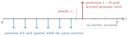
With quarterly premium dates $t_k$ and a default in $(t_{k-1},t_k]$ settled at $t_k$ with half a period of accrued premium, the two legs on a discount curve $P$ and a survival curve $Q_C$ are

\begin{align*} \text{premium} &= \mathcal S\sum_k\delta_kP(0,t_k)\Bigl(Q_C(t_k)+\tfrac12\bigl(Q_C(t_{k-1})-Q_C(t_k)\bigr)\Bigr),\\ \text{protection} &= (1-R)\sum_kP(0,t_k)\bigl(Q_C(t_{k-1})-Q_C(t_k)\bigr). \end{align*}

The half-period accrual stands for the premium the buyer owes from the last payment date to the default; the settlement at the period end instead of at default is a small discounting error that the standard model removes by integrating over default times. Figure 13.1 shows the two legs as cash-flow streams.

**Figure 13.1.** The two legs of a default swap. The buyer pays the premium quarterly (blue) until default; at default the seller pays the loss given default and the buyer the premium accrued since the last payment (red). Schematic.

def legs(curve: HazardCurve, disc, maturity: float, recovery: float = 0.4, freq: int = 4) -> tuple[float, float]:
    """(risky annuity per unit of running coupon, protection leg) with defaults settled at period ends."""
    dt, ann, prot = 1.0 / freq, 0.0, 0.0
    for k in range(1, round(maturity * freq) + 1):
        q0, q1 = curve.survival((k - 1) * dt), curve.survival(k * dt)
        df = disc.df_t(k * dt)
        ann += dt * df * (q1 + 0.5 * (q0 - q1))
        prot += (1.0 - recovery) * df * (q0 - q1)
    return ann, prot

Listing 13.1. The risky annuity and the protection leg on a discount curve and a hazard curve. code/firm/cdscurve/firm_cdscurve.py

13.3 Bootstrapping a hazard curve

Method 13.6 (Hazard curve from par spreads)

Take par spreads for increasing maturities $T_1<T_2<\dots$ and a recovery rate. Solve for a constant hazard on $(0,T_1]$ that reprices the first; holding it, a constant hazard on $(T_1,T_2]$ that reprices the second; and so on. The survival curve is $Q_C(t) = e^{-\int_0^t\lambda}$ with the piecewise-constant hazards. Check that each input reprices and that no hazard is negative (a negative hazard means the quotes are inconsistent).

def bootstrap(disc, tenors: Sequence[float], spreads: Sequence[float], recovery: float = 0.4) -> HazardCurve:
    """Piecewise-constant hazards, one per tenor, so that each par CDS reprices (bisection)."""
    times, hz = [], []
    for T, s in zip(tenors, spreads, strict=True):
        times.append(T)
        hz.append(0.0)
        lo, hi = 0.0, 3.0
        for _ in range(100):
            mid = 0.5 * (lo + hi)
            hz[-1] = mid
            lo, hi = (mid, hi) if par_spread(HazardCurve(times, hz), disc, T, recovery) < s else (lo, mid)
        hz[-1] = 0.5 * (lo + hi)
    return HazardCurve(times, hz)

Listing 13.2. Bootstrapping piecewise-constant hazards so that every par default swap reprices. code/firm/cdscurve/firm_cdscurve.py

Example 13.7 (An investment-grade curve)

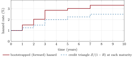
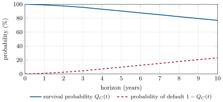
Par spreads of 60, 75, 90, 120, 135 and 150 basis points at one, two, three, five, seven and ten years (illustrative), recovery 40%, on chapter 1’s SOFR curve, bootstrap to hazards of 1.00%, 1.51%, 2.04%, 2.86%, 3.03% and 3.32% on the successive intervals (Figure 13.2). The credit triangle gives 1.00%, 1.25%, 1.50%, 2.00%, 2.25% and 2.50%: the average hazard to each maturity, where the bootstrap gives the forward hazard on each interval. The probability of default is 0.995% over one year, 9.76% over five and 23.1% over ten (Figure 13.3).

**Figure 13.2.** The hazard curve bootstrapped from six par spreads, and the average hazard the credit triangle reads from each spread. An upward-sloping spread curve means higher forward hazards further out. Data: illustrative spreads on chapter 1’s curve; the chapter’s tutorial.

**Figure 13.3.** Survival and default probabilities of the bootstrapped name to ten years. The survival curve bends down faster as the forward hazard rises; the probability of default reaches 9.8% at five years and 23.1% at ten. Data: the chapter’s tutorial.

Remark 13.8 (Recovery is a convention, expected loss is not)

Spreads pin down the expected loss, roughly $\lambda(1-R)$ , not the hazard alone. With a recovery of 25% instead of 40% the same spreads bootstrap to hazards of 0.80% to 2.64% and a five-year probability of default of 7.87% instead of 9.76%, while every quoted swap is worth the same. Recovery matters for positions that are not par swaps: a bond priced near par, a swap far from its coupon, and the jump-to-default of any of them.

Remark 13.9 (Inconsistent quotes)

If the three-year spread were 50 basis points, below the two-year 75, repricing it would need a negative hazard on the third year: the bisection of Listing 13.2 stops at zero and reprices only 51.0 basis points. A curve that fails this check is telling the desk that one quote is stale, or that the recovery assumed is wrong.

13.4 The standard model and its conventions

Definition 13.10 (ISDA standard model)

The ISDA standard model is the open-source reduced-form pricer, with agreed conventions (a flat hazard implied from a quoted spread, a standard recovery, the day’s standard discount curve, accrual and payment rules), that the market uses to convert between a contract’s quoted spread and the upfront payment at its standard coupon.

A quoted spread of a standard contract is thus not a par spread of a bootstrapped curve: it is the flat spread that, in the standard model, gives the traded upfront. The two agree for the maturity quoted and differ for positions of other maturities, which a desk values on its bootstrapped curve.

Example 13.11 (Upfront at a standard coupon)

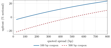
The five-year contract quoted at 120 basis points with a 100-basis-point coupon costs the protection buyer an upfront of 0.872% of notional (flat hazard from the quote, the five-year zero rate of 3.42% flat, recovery 40%). A name quoted at 500 has no upfront at the 500 coupon and one of 15.06% at the 100 coupon (Figure 13.4).

**Figure 13.4.** Upfront paid by the protection buyer of a five-year standard contract, from the quoted spread, at the two North American standard coupons. The upfront is zero where the quote equals the coupon and negative (received) below it. Data: the standard flat-hazard conversion; the chapter’s tutorial.

As of September 2026 — Standard contracts

Since the Big Bang Protocol of 8 April 2009, North American single-name default swaps trade with a 100-basis-point coupon on investment-grade names and 500 on high-yield names, with an upfront settling the difference, and settle credit events by auction. The standard model used for the conversion is published as open-source code under an ISDA licence and administered by S&P Global Market Intelligence.

13.5 Bonds on the hazard curve

The same survival curve prices a fixed-coupon bond of the name: each coupon is a risky discount factor, and default pays the recovery rate on the face value (recovery of par) at the period end, as in risky_bond. The value of a bond on the hazard curve bootstrapped from default swaps, compared with its market price, gives the difference between the two markets’ prices of the same credit.

Example 13.12 (A five-year bond on the curve)

A five-year 5% bond of the name (semi-annual coupons) is worth 107.08 per 100 on the riskless curve and 101.38 on the bootstrapped hazard curve. The risky discount factor to five years is 0.7604, against a riskless 0.8427. If the bond trades at 97.00, the flat hazard that reprices it corresponds to a default-swap spread of 220 basis points: the bond is 100 basis points cheaper than the default swap says, a negative basis of $-99.8$ basis points (default swap minus bond-implied spread).

A negative basis invites buying the bond and buying protection: the package collects the bond’s excess spread while the protection covers default. It is not an arbitrage: it must be funded, it is marked to a basis that can widen, and its default payoff depends on the hedge ratio and on the recovery; the weekend problem measures it.

13.6 Credit risk measures: CS01 and jump to default

Definition 13.13 (CS01)

The CS01 of a position is the change in its value when a credit spread rises by one basis point: bucketed, per quoted maturity with the hazard curve re-bootstrapped, or parallel.

Definition 13.14 (Jump-to-default risk)

Jump-to-default risk (JTD) is the change in a position’s value if the name defaults now: the protection paid or received, $\pm(1-R)N$ , minus the position’s current value, which disappears. It is not captured by CS01: default is a jump, not a large spread move.

Example 13.15 (A protection position)

Long USD 10 million of five-year protection at the 100 coupon on the curve of Example 13.7: worth USD 88 133 (the risky annuity is 4.41), with a CS01 of USD 4 391 on the five-year quote and almost nothing elsewhere, and a jump-to-default gain of USD 5.91 million.

Definition 13.16 (Default risk premium)

The default risk premium is the difference between the risk-neutral default probability implied by spreads and the real-world probability estimated from default histories: spreads pay for expected losses, for their uncertainty and for the illiquidity of credit, so implied PDs exceed historical ones, most for high-quality names.

Remark 13.17 (Which PD to use)

Pricing and hedging use the risk-neutral PD (9.76% over five years above); capital models, provisions and ratings use real-world PDs. If the real-world five-year PD of the name were 1.5%, spreads would price more than six times the expected default losses. Hull, Predescu and White (2005) found seven-year risk-neutral default intensities 16.8 times the historical ones for Aaa bonds, 9.8 for A, 5.1 for Baa, 2.1 for Ba and 1.2 for B.

13.7 Tutorial: a hazard curve

Goal. Bootstrap a hazard curve from par spreads, convert quotes to upfronts, and measure a position’s CS01 and jump-to-default. End state: Figures 13.2 and 13.4 and the numbers of Examples 13.7 and 13.15.

Bootstrap: bootstrap(disc, tenors, spreads, recovery); check each par spread reprices.
Triangle: hazard_table() against $\mathcal S/(1-R)$ .
Upfronts: standard_upfront (Book 2’s flat-hazard conversion).
Risk: protection_position(); fig_rc_credit.py writes the charts.

What to change next. Use a recovery of 25% and compare hazards and upfronts; make the three-year spread 50 basis points and watch the bootstrap fail to reprice it (Remark 13.9).

13.8 Build: the credit curve

Purpose. The credit curves of the miniature firm: every default swap, credit bond and counterparty in chapters 14 to 20 reads a hazard curve built here.

Interface. HazardCurve(times, hazards) with cum and survival; legs, par_spread, bootstrap; standard_upfront; cds_value; risky_bond; bucketed_cs01; jump_to_default.

Rules. Quarterly premiums with half-period accrual on default, defaults settled at period ends; any discount curve with df_t; Book 2’s firm_cds for the flat conversion.

Acceptance tests. code/firm/cdscurve/tests/: every quote reprices; one tenor gives Book 2’s flat hazard; the upfront vanishes at the coupon; a bond with zero hazard is a riskless bond; CS01 falls on the position’s own maturity; jump-to-default of a protection buyer is $(1-R)N$ minus its value.

Stretch. Business-day schedules and the standard model’s exact conventions (step-in, protection from trade date); recovery-rate risk; stochastic intensity.

Sources and further reading

Paul, Weiss, “The Big Bang Protocol and a new structural framework for credit default swaps”, 24 March 2009.
ISDA CDS Standard Model, cdsmodel.com.
D. O’Kane, Modelling Single-name and Multi-name Credit Derivatives, Wiley, 2008, chapters 3–7.
J. Hull, M. Predescu and A. White, “Bond prices, default probabilities and risk premiums”, Journal of Credit Risk 1(2), 2005, 53–60.

13.9 Exercises

Exercise 13.1 ★

A name’s five-year spread is 180 basis points and recovery 40%. Estimate its hazard rate and five-year survival probability with the credit triangle.

Solution

Solution of Exercise 13.1.

$\lambda \approx 0.0180/0.60 = 3.00\%$ a year; five-year survival $e^{-0.03\times5} = 86.07\%$ , a probability of default of 13.9%.

Exercise 13.2 ★

Why is a bootstrapped hazard higher than the triangle’s hazard when the spread curve slopes upward?

Solution

Solution of Exercise 13.2.

Each spread prices the average hazard up to its maturity. When spreads rise with maturity, the later interval must carry a higher hazard than the average so far to lift the average: forward hazards lie above average hazards, as forward rates lie above zero rates on an upward-sloping curve.

Exercise 13.3 ★

In Example 13.15, what is the jump-to-default of the seller of the same protection?

Solution

Solution of Exercise 13.3.

The seller pays $(1-R)N = \text{USD}~6$ million and loses its position, worth $-\text{USD}~88\,133$ to it: the jump-to-default is $-6\,000\,000+88\,133 = -\text{USD}~5\,911\,867$ , the mirror image of the buyer’s.

Exercise 13.4 ★★

Estimate the CS01 of the protection position from its risky annuity, and compare with USD 4 391.

Solution

Solution of Exercise 13.4.

A one-basis-point rise in the spread raises the protection buyer’s value by about the risky annuity times the notional times $10^{-4}$ : $4.41\times10\,000\,000\times10^{-4} \approx \text{USD}~4\,407$ , close to the bucketed USD 4 391. The difference is the fall of the annuity itself as the hazard rises.

Exercise 13.5 ★★

A high-yield name is quoted at 350 basis points. Give the five-year upfront at the 500 coupon with the chapter’s conventions, say who pays it, and give the upfront at the 100 coupon.

Solution

Solution of Exercise 13.5.

At the 500 coupon the quote is below the coupon, so the buyer receives an upfront of 5.98% of notional (an upfront of $-5.98\%$ paid by the buyer); at the 100 coupon the buyer would pay 9.96%.

Exercise 13.6 ★★

Why is jump-to-default not the CS01 times a very large spread move?

Solution

Solution of Exercise 13.6.

CS01 is a derivative: it describes small, continuous changes of spreads while the name survives. Default is a jump of the default indicator: the protection pays a fixed loss and the position’s premium stream stops, whatever the spread was just before. Spreads blowing out to thousands of basis points approach but never reach the default payoff, and a linear extrapolation of CS01 overshoots or undershoots it depending on the position.

Exercise 13.7 ★★★

Coding. Compute the negative-basis package of the weekend problem: the bond-implied spread, the basis, and the package’s jump-to-default with a par-for-par hedge.

Solution

Solution of Exercise 13.7.

basis_package(): the bond-implied spread is 220 basis points, the basis $-99.8$ basis points, and the jump-to-default with USD 100 million of protection $100\text{m}\times(0.40-0.97)+100\text{m}\times0.60-88\,133\times10 = \text{USD}~2\,118\,667$ .

Exercise 13.8 ★★★

Find the flaw. “The five-year spread is 120 basis points, so the market thinks the name has a 2% chance of defaulting each year.”

Solution

Solution of Exercise 13.8.

Two flaws. The credit triangle gives a hazard of $0.0120/0.60 = 2\%$ only for a recovery of 40%, and a flat curve; with this chapter’s upward-sloping curve the one-year hazard is 1.00%. And the probabilities in spreads are risk-neutral: they include the default risk premium, so the market’s real-world estimate of default is lower.

13.10 Problem: The Negative Basis Package

Problem 13.1

Weekend problem — buying a cheap bond with protection

The chapter’s name has a five-year 5% bond (semi-annual) trading at 97.00 while its five-year default swap is quoted at 120 basis points. A fund buys USD 100 million face of the bond and five-year protection at the 100 coupon.

Part I — The basis.

Give the bond’s value on the bootstrapped hazard curve.
Give the flat par spread that reprices the bond at 97.00.
Give the basis (default swap minus bond-implied spread).
Why might a bond trade so far below its default-swap-implied value?
What does the fund earn if nothing happens?

Part II — Hedge ratios.

Give the jump-to-default with USD 100 million of protection (par for par).
Give it with USD 97 million (market value).
Give the package’s CS01 in each case.
Give the recovery at which the market-value package breaks even on default.
Which hedge would you choose, and why?

Part III — Risks.

What happens to the package if the basis widens further?
What funding risk does the fund carry?
What is the cheapest-to-deliver option in the default swap worth to the fund?
What counterparty risk does the protection carry?
How would the package behave in a 2008-style dash for cash?

Part IV — Judgement.

Why is the negative basis called an arbitrage, and why is it not one?
Which desks run it, and with what balance sheet?
What would you ask before putting it on?
State the named result: the basis, and the package’s jump-to-default and CS01 with the par-for-par hedge.
In one sentence: what does a negative basis measure?

Solution

Solution of Problem 13.1.

1. 101.38 per 100. 2. 220 basis points. 3. $120-220 = -99.8$ basis points (to one decimal). 4. The bond must be funded and financed (repo haircuts, balance sheet), it may be illiquid or in forced selling, the bond and swap may reference different deliverables, and in 2008 funding costs dwarfed default risk. 5. The bond’s yield over funding, less the protection coupon, plus the pull of the basis to zero if it converges; the upfront paid on the protection is part of the cost. 6. USD 2 118 667. 7. USD 345 107. 8. $-\text{USD}~2\,141$ (par for par) and $-\text{USD}~3\,453$ (market value) per basis point. 9. 28.5%. 10. Par for par hedges the face that the default swap delivers against, so the package gains on default at any recovery; the market-value hedge is cheaper and leaves less spread risk but loses on default below 28.5% recovery. Funds that can tolerate spread risk choose par for par. 11. The package marks down: the bond falls more than the protection gains, through the negative CS01, although the carry is unchanged if held to maturity. 12. The bond is financed in repo; a rise in haircuts or repo rates, or a withdrawn line, forces a sale at the widest basis. 13. On default the buyer can deliver the cheapest deliverable obligation; settlement by auction sets one final price for all, which reduces the option’s value, but a package long a bond trading above the auction price still earns the difference. 14. The seller may default together with the name or in a crisis: the protection is worth least when it is needed. Clearing removes most of it for standard contracts. 15. Holders sell bonds to raise cash, the basis widens sharply, repo tightens, and the package marks down while nothing has defaulted, as in the fourth quarter of 2008. 16. It is riskless on default and to maturity, but its value, funding and margin in between are not, and a leveraged holder can be forced out before convergence. 17. Bank credit desks and relative-value funds with cheap, stable funding and room on the balance sheet; the capital cost of holding the bond decides who can run it. 18. Funding and its term, the deliverables, the counterparty and clearing of the protection, the recovery assumption, and the basis’s history in stress. 19. Named result: the negative-basis package: a basis of $-99.8$ basis points, and with the par-for-par hedge a jump-to-default gain of USD 2 118 667 and a CS01 of $-\text{USD}~2\,141$ per basis point on USD 100 million. 20. What it costs to fund and hold a bond compared with holding the same credit risk unfunded, in a swap.

13.11 Interview questions

Interview question 13.1 ★ trader, researcher

State the credit triangle and use it on a 200-basis-point spread.

Solution

Solution of Interview question 13.1.

Spread $\approx$ hazard $\times$ loss given default. At 200 basis points and 40% recovery the hazard is $0.02/0.6 = 3.33\%$ a year, a five-year survival of about $e^{-0.167} = 84.6\%$ .

What the interviewer is looking for: the formula, its assumptions (flat hazard, continuous premium) and a quick number.

Interview question 13.2 ★★ researcher, developer

How do you bootstrap a hazard curve, and what can go wrong?

Solution

Solution of Interview question 13.2.

Take par spreads for increasing maturities and a recovery; solve for a piecewise-constant hazard interval by interval so that each swap reprices, on a given discount curve. Things that go wrong: inconsistent quotes needing negative hazards, stale quotes, the recovery assumption, interpolation choices between pillars, and the sensitivity of forward hazards to small quote changes.

What the interviewer is looking for: the procedure, the positivity check and the role of recovery.

Interview question 13.3 ★★ trader, bank

What changed with the 2009 standardisation of default swaps, and why did it need a common model?

Solution

Solution of Interview question 13.3.

Fixed coupons of 100 and 500 basis points with an upfront, quarterly standard dates, auction settlement of credit events and central clearing. Fixed coupons make contracts on a name fungible so that offsetting trades net; the upfront must be computed identically by both sides and by the clearing house, hence one model with agreed conventions.

What the interviewer is looking for: fungibility, netting and why the conversion must be common.

Interview question 13.4 ★★ risk

Why report jump-to-default separately from CS01?

Solution

Solution of Interview question 13.4.

Default is a jump, not a spread move: CS01 measures small moves while the name survives, whereas jump-to-default is the loss if it defaults now. A book flat CS01 across names can be very long or short default (a short-dated long protection against a long-dated short), and concentration limits and capital rules measure jump-to-default separately.

What the interviewer is looking for: the distinction and a CS01-flat, JTD-long example.

Interview question 13.5 ★★★ researcher, risk

Risk-neutral default probabilities are several times historical ones. Explain, and say which you would use for pricing, provisioning and capital.

Solution

Solution of Interview question 13.5.

Spreads compensate for expected losses, for the uncertainty and correlation of defaults (which cluster in bad times), for liquidity and for funding; risk-neutral probabilities absorb all of it. Pricing and hedging use risk-neutral probabilities; provisioning and capital use real-world estimates (through the cycle or point in time).

What the interviewer is looking for: the default risk premium and the right measure per use.

Interview question 13.6 ★★★ trader

A bond trades 100 basis points wide of its default swap. How do you trade it, and what could go wrong?

Solution

Solution of Interview question 13.6.

Buy the bond and buy protection (a negative-basis package), sized par for par or on market value; finance the bond in repo. It can go wrong through funding, a further widening of the basis marked to market, deliverability, recovery and the protection seller’s risk.

What the interviewer is looking for: the package, the hedge ratio and the funding risk.

Terms defined in this chapter

See all 2333 terms in the glossary