Rates, Credit, XVA and Risk · Rates, credit & risk
9Bermudans and Callables
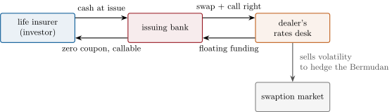
In 2014 Taiwan’s legislature exempted foreign-currency bonds listed on the island from the cap on its life insurers’ overseas investments, and the insurers, with hundreds of billions of dollars to place, began buying thirty-year dollar zero-coupon bonds that the issuing banks could call every year after the first few. The investors earned a yield well above the Treasury curve for selling that right. The issuers did not keep it: they swapped each bond into floating funding with a dealer, and the swap carried the call, so that dealers ended up long a large stock of Bermudan options on long-dated rates. To hedge, they sold volatility in the swaption market, year after year. The instrument at the centre is the Bermudan swaption: an option to enter a swap on any one of several dates. It is worth more than the most valuable of the Europeans it can become, by an amount no European hedge captures. This chapter prices it on chapter 7’s tree and by regression Monte Carlo, measures that amount, and prices the callable zero-coupon bond the insurers bought.
9.1 Bermudan swaptions and their co-terminal Europeans
Definition 9.1 (Bermudan swaption)
A Bermudan swaption gives the right, on any one of a set of exercise dates , to enter the swap that starts on that date and ends on a fixed final date , at a fixed rate . A “ten-non-call-one” receiver Bermudan can be exercised every year from year one into a receiver swap ending at year ten. It is a Bermudan exercise right in the sense of One Quant Book 5, chapter 6, applied to swaps.
Definition 9.2 (Co-terminal swaption)
The co-terminal swaptions of a Bermudan are the European swaptions expiring on each of its exercise dates into the swap ending on its final date: the Europeans it can become.
Definition 9.3 (Switch option)
The switch option of a Bermudan is its value minus the value of its most expensive co-terminal European: the value of being able to choose the exercise date after seeing the rates.
Proposition 9.4 (Bounds from the Europeans)
A Bermudan is worth at least its most expensive co-terminal European and at most the sum of all of them.
Proof. The holder can commit to one exercise date, which gives the European; any exercise policy exercises on at most one date, so the payoff is dominated by the sum of all the Europeans’ payoffs. ∎
The lower bound is what a static hedge with Europeans secures; the switch option depends on how the co-terminal swap rates move together, which only a model of the whole curve can price.
9.2 Exercise by backward induction on a tree
Method 9.5 (A Bermudan on the Hull–White tree)
Build chapter 7’s tree to the final date. Roll back from the last exercise date: at each exercise date, compute at every node the value of the underlying swap (its zero-coupon bonds rolled back on the tree), and replace the continuation value by the maximum of the two; between exercise dates, discount along the branches. The value at the root is the Bermudan’s price; the nodes where exercise wins trace the exercise boundary.
def bermudan_tree(tree: HWTree, exercises: Sequence[int], final: int, K: float, receiver: bool = True) -> float:
    """Bermudan swaption by backward induction: exercise at year e into the swap from e to final."""
    per = int(round(1.0 / tree.dt))
    final_step = final * per
    ex_steps = {e * per: e for e in exercises}
    v = np.zeros(2 * tree.jmax + 1)
    for i in range(max(ex_steps), -1, -1):
        if i in ex_steps:
            sw = _swap_values_on_tree(tree, i, final_step, per, K)
            v = np.maximum(v, sw if receiver else -sw)
        if i > 0:
            v = tree.step_back(v, i - 1)
return float(v[tree.jmax])Example 9.6 (A ten-non-call-one receiver)
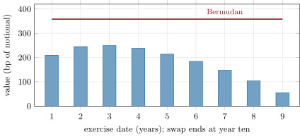
On chapter 2’s euro OIS curve, with Hull–White at and basis points (chapter 7’s single-volatility fit), a receiver Bermudan at the ten-year par rate of 2.585% exercisable every year from one to nine is worth 358.4 basis points of notional. Its co-terminal Europeans are worth 209.5, 245.3, 249.5, 237.8, 214.1, 184.3, 147.8, 104.3 and 54.9 basis points (tree, within 1.4 of Jamshidian’s formula; Figure 9.1); the most expensive is the three-year. The switch option is worth 109.0 basis points, 44% of the best European.
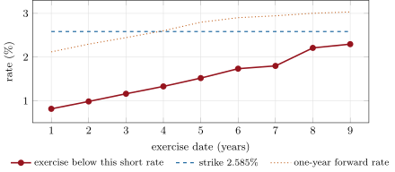
The exercise boundary of the receiver is a short rate below which exercising beats waiting (Figure 9.2). Early on the rate must fall far, to 0.82% in year one, since exercising gives up eight more chances; by year nine exercise is worth it below 2.30%, close to the strike.
Example 9.7 (Mean reversion and the switch)
Recalibrating so that the five-into-five European keeps its price, the Bermudan and its switch option depend on (table below): stronger mean reversion decorrelates the rates of successive exercise dates and makes the choice of date more valuable, while the best European barely moves.
| (bp) | Bermudan (bp) | best European (bp) | switch (bp) | |
|---|---|---|---|---|
| 1% | 78.1 | 351.0 | 249.2 | 101.9 |
| 3% | 86.0 | 358.4 | 249.5 | 109.0 |
| 6% | 98.9 | 369.7 | 249.7 | 120.0 |
9.3 Exercise by regression in Monte Carlo
Trees serve one or two factors; a market model (chapter 8) or any model with many state variables is simulated, and simulation runs forward while exercise is decided backward. The Longstaff–Schwartz method (One Quant Book 5, chapter 23) estimates the continuation value by regressing, at each exercise date, the discounted future cash flows of in-the-money paths on functions of the state.
Method 9.8 (Regression exercise for a Bermudan swaption)
Simulate the state under a convenient measure (here the terminal forward measure of year ten, numeraire ) at the exercise dates. From the last date back: compute the exercise value in numeraire units; on in-the-money paths regress the realised future cash flow on , the exercise value and its square; exercise where the exercise value beats the fitted continuation. Fit the regressions on one set of paths and apply the rule to an independent set: the result is a price of a feasible policy, hence a lower bound.
    def run(seed_, coefs=None):
        xs = simulate_x(m, float(final), times, paths, seed=seed_)
        cf = np.zeros(paths)                                   # deflated cash flow of the policy
        fitted = {}
        for e in sorted(exercises, reverse=True):
            x = xs[float(e)]
            ex = _swap_value_x(m, e, final, K, x) / _numeraire_x(m, e, final, x)
            itm = ex > 0
            if e == max(exercises):
                cf = np.where(itm, ex, 0.0)
                continue
            basis = np.column_stack([np.ones(itm.sum()), ex[itm], ex[itm] ** 2])
            if coefs is None:
                beta, *_ = np.linalg.lstsq(basis, cf[itm], rcond=None)
                fitted[e] = beta
            else:
                beta = coefs[e]
            cont = basis @ beta
            exercise_now = np.zeros(paths, bool)
            exercise_now[np.flatnonzero(itm)[ex[itm] > cont]] = True
            cf = np.where(exercise_now, ex, cf)
return cf, fittedExample 9.9 (Tree and regression agree)
With 40 000 paths under the ten-year forward measure (antithetic, half-monthly steps) the regression price of the ten-non-call-one is 358.1 basis points with a standard error of 1.9, against 358.4 on the tree.
9.4 Upper bounds and the switch option
A regression price is a lower bound; how far below the true value it lies is measured by a dual upper bound (One Quant Book 5, chapter 23), which subtracts a martingale from the payoff and takes the maximum over dates along each path: the gap between the two bounds certifies the policy, and computing it (by nested simulation) belongs in the pricer’s validation. Once the gap is small, the practical risks lie elsewhere: in the model’s correlation and volatility structure, which set the switch option’s size.
Remark 9.10 (Hedging a Bermudan)
A Bermudan’s vega sits on its co-terminal swaptions, split roughly in proportion to the probability of exercising into each; its switch option is a bet on the decorrelation of successive swap rates that no European captures. Desks hedge the Europeans’ vega and carry, with a reserve, the rest; a change of model (chapter 7’s , a market model’s ) moves the switch value.
9.5 The callable-bond issuance business
Definition 9.11 (Formosa bond)
A Formosa bond is a bond denominated in a foreign currency and issued and listed in Taiwan. From 2014 most dollar Formosas were long-dated (twenty or thirty years) and callable by the issuer, many with zero coupons, sold to Taiwanese life insurers.
Definition 9.12 (Callable range accrual)
A callable range accrual is a callable note whose coupon accrues only on days when a reference rate stays within a range; the issuer’s call makes it a Bermudan on a portfolio of digital options, and it is priced with the same exercise methods, on a model that also fits the smile.
As of September 2026 — The Formosa market
In May 2014 Taiwan’s legislature excluded locally issued foreign-currency bonds from the 45% cap on insurers’ overseas investments, unlocking funds reported at USD 586 billion; the dollar notes sold in the following months were all callable, with maturities of twenty or thirty years, and 74% paid no coupon (Bloomberg data). The trade press has described the resulting hedging flows as a steady supply of long-dated dollar volatility that helped hold it down.
9.6 Tutorial: a Bermudan three ways
Goal. Price a ten-non-call-one receiver on the tree and by regression, measure its switch option and its exercise boundary. End state: Figures 9.1 and 9.2 and the numbers of Examples 9.6 and 9.9.
- Tree:
bermudan_summary()builds chapter 7’s tree with half-monthly steps and prices the Bermudan and its nine Europeans. - Boundary:
boundary(). - Regression:
lsm_check()on 40 000 paths. - Mean reversion:
mean_reversion_table();fig_rc_bermudan.pywrites the charts.
What to change next. Add and the one-year rate to the regression basis and see whether the price rises; price the Bermudan on chapter 7’s piecewise- model with Monte Carlo.
9.7 Build: Bermudan and callable pricers
Purpose. The book’s callable products: Bermudan swaptions, callable bonds and notes, and the exercise decisions of chapter 12’s mortgages.
Interface. bermudan_tree(tree, exercises, final, K, receiver); exercise_boundary; callable_zero_tree(tree, maturity, accretion, calls); simulate_x, bermudan_lsm(model, exercises, final, K, paths); switch_option.
Rules. Chapter 7’s firm_shortrate imported; regression fitted and applied on independent path sets; fixed seeds; numpy only.
Acceptance tests. code/firm/bermudan/tests/: a single exercise date gives the European; the Bermudan lies between the best European and the sum; regression agrees with the tree; a zero accreting far above rates is called at the first date and one accreting at zero almost never; the boundary lies below the strike.
Stretch. A dual upper bound by nested simulation; Bermudans in the market model of chapter 8; callable range accruals.
Sources and further reading
- F. Longstaff and E. Schwartz, “Valuing American options by simulation: a simple least-squares approach”, Review of Financial Studies 14(1), 2001.
- L. Andersen and M. Broadie, “Primal-dual simulation algorithm for pricing multidimensional American options”, Management Science 50(9), 2004.
- Insurance Journal (Bloomberg News), “Goldman leads Wall Street tapping Taiwan cash pile”, 10 September 2014; Risk.net, “Formosas, the Fed, and the billion-dollar Bermudan trade”.
- L. Andersen and V. Piterbarg, Interest Rate Modeling, volume 3, Atlantic Financial Press, 2010, chapter 19.
9.8 Exercises
Exercise 9.1 ★
Using Example 9.6, give the lower and upper bounds of Proposition 9.4 and check the Bermudan lies between them.
Solution
Solution of Exercise 9.1.
Lower bound: the three-year European, 249.5 basis points. Upper bound: the sum of the nine, 1 647.5. The Bermudan, 358.4, lies between, much nearer the lower bound.
Exercise 9.2 ★
Why is the three-year European the most expensive, and not the one-year with the longest swap?
Solution
Solution of Exercise 9.2.
A European’s value is roughly annuity times volatility times the square root of expiry: the one-year has the longest swap (largest annuity) but little time for rates to move; the nine-year has time but a one-year swap. The product peaks at three years here.
Exercise 9.3 ★
An investor buys a thirty-year callable zero instead of a straight one. What has she sold, and to whom does it end up?
Solution
Solution of Exercise 9.3.
She has sold the issuer a Bermudan option to redeem at the accreted value, a receiver-type option on long rates (the issuer calls when rates fall). The issuer passes it through the swap to the dealer, who hedges it by selling swaption volatility to the market.
Exercise 9.4 ★★
Read Figure 9.2. Why does the boundary rise towards the strike, and why does it stay below the one-year forward rate?
Solution
Solution of Exercise 9.4.
With fewer exercise dates left, waiting is worth less, so exercise needs a smaller move in the holder’s favour; at the last date the Bermudan is a European and exercise happens whenever the swap is in the money. The boundary stays below the forward because at the money the continuation value (option on later dates) exceeds the immediate intrinsic value.
Exercise 9.5 ★★
Explain, from the table of Example 9.7, why the switch option rises with while the best European barely changes.
Solution
Solution of Exercise 9.5.
The best European is held fixed by recalibrating on the five-into-five, so it moves little. Stronger mean reversion makes swap rates of different exercise dates less correlated: a low rate at year three says less about year six, so the right to choose the date later is worth more (101.9, 109.0 and 120.0 basis points).
Exercise 9.6 ★★
Why must the regression be fitted on one set of paths and applied to another to give a lower bound?
Solution
Solution of Exercise 9.6.
Fitted and applied on the same paths, the regression uses each path’s own future to decide whether to exercise, a look-ahead that biases the price upward; applied to independent paths, the rule is a legitimate (sub-optimal) stopping rule, whose expected payoff is a lower bound.
Exercise 9.7 ★★★
Coding. Price the thirty-non-call-five callable zero of the weekend problem at its par accretion yield, and find the yield of the straight zero on the same curve.
Solution
Solution of Exercise 9.7.
The callable zero is worth par at an accretion yield of 5.61%; the straight thirty-year zero on the curve yields 4.13% (annual). The investor earns 1.48 percentage points a year for the call.
Exercise 9.8 ★★★
Find the flaw. “We hedge our Bermudan with the most expensive co-terminal European, in the same notional, so we are hedged.”
Solution
Solution of Exercise 9.8.
The European covers only the lower bound: the switch option (here 44% of the best European) is unhedged, and the vega of the Bermudan is spread over all the co-terminals, shifting as rates move; the notional of a delta- and vega-neutral hedge is not the Bermudan’s notional. Hedge each co-terminal’s vega and delta, and reserve for the switch.
9.9 Problem: The Formosa Hedge
Problem 9.1
Weekend problem — a thirty-year callable zero
A bank issues a thirty-year dollar zero-coupon Formosa bond, callable every year from year five at its accreted value, and sells it at par to a life insurer. It swaps the bond with a dealer, who takes over the call. Price it with Hull–White (, basis points) on chapter 1’s SOFR curve (monotone convex), monthly tree.
Part I — The bond.
- Give the thirty-year zero-coupon yield of the curve (annual compounding).
- Give the accretion yield at which the callable zero is worth par.
- Give the value of the straight zero at that accretion, per unit issued.
- Give the value of the issuer’s call.
- Why does the investor accept this?
Part II — The option.
- Which single call date is worth the most as a European, and how much?
- Give the Bermudan premium over that European.
- Why is the first call date the most valuable European here?
- What is the dealer long, and against what?
- Why does the dealer not simply keep the option?
Part III — The hedge.
- Give the vega of the call per basis point of volatility, per USD 1 billion.
- Which swaptions does the dealer sell to hedge it?
- If ten such issues of USD 1 billion come in a month, what vega enters the market?
- What happens to long-dated swaption volatility, and to the dealers’ marks?
- When rates fall and the bonds are called, what happens to the hedges?
Part IV — Judgement.
- What risks does the insurer keep?
- Why is the trade concentrated in few dealers, and why does that matter?
- What model risk does the dealer carry?
- State the named result: the par accretion yield, the Bermudan premium over the best European and the vega per USD 1 billion.
- In one sentence: who sells volatility in this chain, and why?
Solution
Solution of Problem 9.1.
1. 4.13%. 2. 5.61%. 3. 1.526. 4. 0.526 per unit issued: 1.526 minus par. 5. For 1.48 percentage points a year of extra yield, and because the regulation made these bonds the most efficient way to hold long dollar duration. 6. Year five, the first call: 0.456. 7. 0.070 per unit. 8. A zero-coupon bond called at its accreted value is most in the money early (the accretion compounds above the curve’s rates from the start), and the first call cuts the longest remaining liability. 9. A Bermudan receiver-type option on long rates, received through the swap from the issuer, against which the dealer pays the floating funding. 10. It is a large long-volatility position in illiquid long-dated options; dealers are paid to warehouse and hedge it, not to hold it. 11. USD 2.33 million per basis point of the model’s per USD 1 billion. 12. Long-dated swaptions (co-terminals of thirty-year swaps from five years on), and longer-expiry receivers. 13. About USD 23.3 million per basis point of . 14. It is pushed down by the steady selling; dealers long the Bermudans mark them lower as volatility falls. 15. The Bermudan disappears when called: the dealer is left short the volatility it sold, and must buy it back, often in a falling-rate, rising-volatility market. 16. Reinvestment risk when called (in low-rate states), currency risk against its liabilities, and concentration in few issuers. 17. Few dealers can warehouse and hedge the options; their hedging is correlated, so the flows move the market and a reversal (calls) hits them all at once. 18. The volatility and correlation structure of the model (the switch value), the smile of long-dated swaptions, and the exercise rule. 19. Named result: the Formosa hedge: the callable zero is at par at an accretion of 5.61% against 4.13% for the straight zero; the Bermudan call is worth 0.070 more than the best European (0.456); its vega is USD 2.33 million per basis point per USD 1 billion. 20. The dealer sells volatility, because it bought a Bermudan it does not want to carry, from an issuer who took it from an investor paid to give it up.
9.10 Interview questions
Interview question 9.1 ★ trader, bank
What is a Bermudan swaption, and why is it worth more than any of its Europeans?
Solution
Solution of Interview question 9.1.
The right to enter, on any one of several dates, a swap ending on a fixed date. It is worth at least any single European (commit to that date) and more, because the holder chooses the date after seeing rates: the switch option.
What the interviewer is looking for: the definition and the switch option.
Interview question 9.2 ★★ researcher, developer
Explain Longstaff–Schwartz for a Bermudan swaption. Why is it a lower bound?
Solution
Solution of Interview question 9.2.
Simulate the state; from the last exercise date back, regress the discounted realised future cash flows of in-the-money paths on basis functions of the state and exercise where the exercise value exceeds the fitted continuation. Any exercise rule gives an achievable payoff, so its value (on paths independent from the fit) is at most the optimum.
What the interviewer is looking for: the backward regression and why it bounds from below.
Interview question 9.3 ★★ researcher
Which parameter of a one-factor model drives the switch option, and how?
Solution
Solution of Interview question 9.3.
Mean reversion: it decorrelates the swap rates of successive exercise dates; with the Europeans’ prices held by recalibrating , higher gives a larger switch option.
What the interviewer is looking for: mean reversion as correlation between exercises.
Interview question 9.4 ★★ trader
Why do callable-bond issuance programmes affect long-dated swaption volatility?
Solution
Solution of Interview question 9.4.
Issuers of callable bonds swap them with dealers and pass on the call; dealers, long Bermudans, hedge by selling long-dated swaptions, a steady supply that depresses long-dated implied volatility; calls or unwinds reverse the flow.
What the interviewer is looking for: the chain from investor to swaption market.
Interview question 9.5 ★★★ researcher, risk
How would you validate a Bermudan pricer?
Solution
Solution of Interview question 9.5.
Compare with Europeans (single-date limit) and bounds; tree against regression on the same model; convergence in steps and paths; a dual upper bound for the gap; sensitivity to model parameters (, , correlation) and to the calibration set; stability of Greeks; benchmark against an independent model.
What the interviewer is looking for: a structured validation plan.
Interview question 9.6 ★★★ developer
Your regression Bermudan price moves by two basis points when you change the seed. Is that acceptable, and what would you do?
Solution
Solution of Interview question 9.6.
With a standard error of about two basis points, a two-basis-point move is noise, not a bug. Report the standard error; use more paths, antithetics or control variates (the Europeans have closed forms), fix the seed and the path set for Greeks (common random numbers), and compare with the tree.
What the interviewer is looking for: standard errors and variance reduction.