Rates, Credit, XVA and Risk · Rates, credit & risk

5SABR in Rates and the Volatility Cube

In 2015 a euro rates desk asked its smile model for the volatility of a receiver swaption struck at minus twenty basis points. The model was SABR, the market’s standard since 2002, in the lognormal form every desk used: its formula takes $\ln(F/K)$ and $(FK)^{(1-\beta)/2}$ , and with a negative strike it had nothing to return. Within months the whole euro market had moved to one of two fixes: add a constant to every rate before applying the formula, or use the version of the model in which rates are normal. Each fix fits the quoted strikes; they disagree about the strikes nobody quotes. This chapter applies SABR (One Quant Book 5, chapter 11) to rates, builds the swaption volatility cube from it smile by smile, interpolates it, and looks where it breaks: at negative strikes, and in the low-strike wing of long expiries, where the formula’s density turns negative.

5.1 SABR in rates: normal SABR and the backbone

A forward swap rate $F$ under its annuity measure has SABR dynamics

dF_t = \alpha_t F_t^{\beta}\,dW_t,\qquad d\alpha_t = \nu\alpha_t\,dZ_t,\qquad d\langle W,Z\rangle_t = \rho\,dt ,

with the parameters $(\alpha,\beta,\rho,\nu)$ of Book 5. Rates desks fix $\beta$ by convention rather than by fit, since $\beta$ and $\rho$ both tilt the smile and a single section cannot separate them; the choice sets the backbone, how the at-the-money volatility moves when the forward moves.

Definition 5.1 (Normal SABR)

Normal SABR is SABR with $\beta=0$ : $dF_t=\alpha_t\,dW_t$ , a rate that is normal given its volatility and may take any sign. Its at-the-money normal volatility does not depend on the level of the forward: the backbone is flat in normal terms.

Proposition 5.2 (The normal-volatility expansion of normal SABR)

To first order in the expiry $T$ (Hagan et al., 2002), the normal implied volatility of normal SABR is

\sigma_N(K) = \alpha\,\frac{\zeta}{x(\zeta)}\Bigl(1+\frac{2-3\rho^2}{24}\,\nu^2T\Bigr), \quad \zeta = \frac{\nu}{\alpha}(F-K),\quad x(\zeta) = \ln\frac{\sqrt{1-2\rho\zeta+\zeta^2}+\zeta-\rho}{1-\rho},

with $\zeta/x(\zeta)=1$ at the money. The smile is a function of $F-K$ only: it moves with the forward, strike for strike in basis points.

Proof. Admitted here. ∎

(Hagan et al., 2002, derive it by singular perturbation; One Quant Book 5, chapter 11, gives the lognormal case.)

def hagan_lognormal(f: float, k: float, t: float, p: Sabr) -> float:
    """Black volatility of the shifted rates F + zeta, K + zeta (Hagan et al. 2002, eq. 2.17a)."""
    f, k = f + p.shift, k + p.shift
    if f <= 0 or k <= 0:
        raise ValueError("shifted forward and strike must be positive")
    a, b, r, n = p.alpha, p.beta, p.rho, p.nu
    fk = (f * k) ** ((1 - b) / 2)
    lfk = math.log(f / k)
    denom = fk * (1 + (1 - b) ** 2 / 24 * lfk**2 + (1 - b) ** 4 / 1920 * lfk**4)
    z = n / a * fk * lfk
    zx = 1.0 if abs(z) < 1e-12 else z / _x(z, r)
    corr = 1 + ((1 - b) ** 2 / 24 * a * a / fk**2 + r * b * n * a / (4 * fk) + (2 - 3 * r * r) / 24 * n * n) * t
    return a / denom * zx * corr


def hagan_normal_beta0(f: float, k: float, t: float, p: Sabr) -> float:
    """Normal volatility of normal SABR (beta = 0): alpha * zeta/x(zeta) * (1 + (2 - 3 rho^2) nu^2 t / 24)."""
    a, r, n = p.alpha, p.rho, p.nu
    z = n / a * (f - k)
    zx = 1.0 if abs(z) < 1e-12 else z / _x(z, r)
    return a * zx * (1 + (2 - 3 * r * r) / 24 * n * n * t)

Listing 5.1. Hagan’s lognormal expansion on shifted rates, and the normal-SABR normal volatility. code/firm/sabrcube/firm_sabrcube.py

5.2 Negative rates and shifted models

Definition 5.3 (Shifted lognormal model, shifted SABR)

A shifted lognormal model with shift $\zeta>0$ makes $F+\zeta$ lognormal, $dF_t=\sigma(F_t+\zeta)\,dW_t$ , so that the rate is bounded below by $-\zeta$ ; options are priced with Black’s formula on $F+\zeta$ and $K+\zeta$ . Shifted SABR applies SABR’s dynamics to $F+\zeta$ , $dF_t=\alpha_t(F_t+\zeta)^\beta\,dW_t$ , and Hagan’s lognormal expansion to the shifted forward and strike.

The shift is a floor on the modelled rate, chosen in advance. It should sit below any rate the market can plausibly reach.

Definition 5.4 (Effective lower bound)

The effective lower bound of a policy rate is the level below which a central bank is not expected to cut, because further cuts would push cash out of the banking system or hurt banks more than they ease conditions. Rates models use it to bound the rate distribution, and a shifted model’s shift must exceed it in magnitude.

As of September 2026 — Where the lower bound has been

The ECB’s deposit rate was negative from June 2014 to July 2022, with a low of $-0.50\%$ from September 2019; the Swiss National Bank’s policy rate was $-0.75\%$ from January 2015 and returned above zero in September 2022; the Bank of Japan’s was $-0.1\%$ from 2016 until 19 March 2024.

Example 5.5 (One smile, three models)

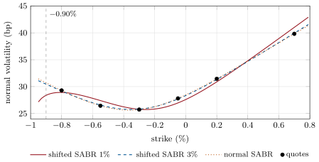
A one-year option on a two-year euro swap, forward $-0.30\%$ , is quoted at normal volatilities of 29.3, 26.5, 25.7, 27.8, 31.4 and 39.8 basis points at strikes 50 and 25 basis points below the forward, at the money, and 25, 50 and 100 above (a smile generated by normal SABR, illustrative). Shifted SABR with $\beta=0.5$ fits it to 0.77 basis points of root-mean-square error with a shift of 1%, to 0.11 with a shift of 3%; normal SABR fits it exactly. Asked for a receiver struck at $-0.90\%$ , sixty basis points below the forward and outside the quotes, they answer 0.177, 0.280 and 0.295 basis points of annuity (Figure 5.1): with a 1% shift the modelled rate cannot fall below $-1\%$ , and the deep receiver is 37% cheaper than with 3%.

A negative-rate smile (one year into two years, forward -0.30\%) fitted by three models, in normal volatility. The 3% shift and normal SABR pass through the quotes; the 1% shift misses them by up to 1.2 basis points and, below them, its volatility falls towards its floor at -1\%. Data: synthetic quotes from normal SABR; the chapter’s tutorial. — **Figure 5.1.** A negative-rate smile (one year into two years, forward $-0.30\%$ ) fitted by three models, in normal volatility. The 3% shift and normal SABR pass through the quotes; the 1% shift misses them by up to 1.2 basis points and, below them, its volatility falls towards its floor at $-1\%$ . Data: synthetic quotes from normal SABR; the chapter’s tutorial.

5.3 Building the cube smile by smile

Definition 5.6 (Swaption matrix)

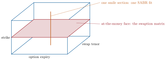
The swaption matrix of a currency is the table of at-the-money swaption volatilities by option expiry and underlying swap tenor: the at-the-money face of the volatility cube (One Quant Book 2, chapter 13).

Method 5.7 (Calibrating the cube)

For each quoted (expiry, tenor): compute the forward swap rate and its annuity on the multi-curve (chapter 2); convert the quotes (normal volatilities, or prices) into the model’s own volatility (shifted Black volatilities for shifted SABR); fix $\beta$ and the shift for the whole currency; fit $(\alpha,\rho,\nu)$ by least squares, with $\alpha>0$ and $|\rho|<1$ imposed by reparametrisation; record the fit error. Then check the parameters for smoothness across the grid: a section whose $\rho$ or $\nu$ jumps is usually a bad quote.

The volatility cube: a smile for each (expiry, tenor). The at-the-money face is the swaption matrix; each vertical line is a section calibrated with its own SABR parameters, and the shift being fixed for the whole currency. — **Figure 5.2.** The volatility cube: a smile for each (expiry, tenor). The at-the-money face is the swaption matrix; each vertical line is a section calibrated with its own SABR parameters, $\beta$ and the shift being fixed for the whole currency.

Example 5.8 (A synthetic euro cube)

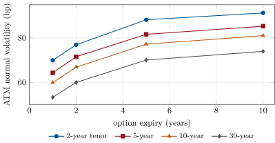
Sixteen sections (expiries one, two, five and ten years; tenors two, five, ten and thirty years), seven strikes each from $-200$ to $+200$ basis points around the forward on chapter 2’s curves, generated by normal SABR with parameters that vary smoothly with expiry and tenor plus seeded noise of 0.3 basis point, are calibrated with shifted SABR ( $\beta=0.5$ , shift 3%). Every section fits to between 0.21 and 0.78 basis point. The at-the-money face (Figure 5.3) rises with expiry and falls with tenor: 69.9 basis points for one year into two, 74.0 for ten into thirty.

**Figure 5.3.** The swaption matrix of the synthetic cube: at-the-money normal volatility of the calibrated sections by expiry, one line per tenor. Data: the chapter’s tutorial.

5.4 Interpolating in expiry, tenor and strike

The cube is quoted on a sparse grid and needed everywhere: a seven-year swap starting in three years, a swaption struck anywhere. The strike dimension is handled by the SABR formula itself; expiry and tenor are handled by interpolating the parameters, not the volatilities, so that every interpolated smile is itself a SABR smile.

Example 5.9 (A section nobody quotes)

Interpolating $(\alpha,\rho,\nu)$ bilinearly in expiry and tenor between the two-, five-year expiries and five-, ten-year tenors gives the three-year into seven-year smile (forward 2.905%) to within 0.93 basis point of the smile the generating parameters imply, over the seven strikes.

Remark 5.10 (What interpolation should respect)

Linear interpolation of $\alpha$ in expiry is a crude rule: total variance, not volatility, should increase with expiry, and $\alpha$ is only the leading term. Desks interpolate in variance along expiry, keep $\rho$ and $\nu$ smooth, and check the interpolated sections for calendar and butterfly arbitrage (One Quant Book 5, chapter 7). Forwards come from the curve, never from interpolation.

5.5 Arbitrage in the wings

Hagan’s formula is an expansion, accurate for moderate $\nu^2T$ and strikes not too far from the forward. Its implied density, the second strike derivative of the call price (Breeden–Litzenberger, One Quant Book 5, chapter 7), can become negative in the low-strike wing of long expiries: a butterfly with negative price.

def density(f: float, t: float, p: Sabr, strikes: Sequence[float], model: str = "shifted",
            h: float = 1e-5) -> list[float]:
    """Implied density of the rate at expiry, d2C/dK2 (per unit annuity), at each strike."""
    return [(price(f, k + h, t, p, model=model) - 2 * price(f, k, t, p, model=model)
             + price(f, k - h, t, p, model=model)) / (h * h) for k in strikes]

Listing 5.2. The implied density of a section, by second differences of prices. code/firm/sabrcube/firm_sabrcube.py

Example 5.11 (Ten years into ten)

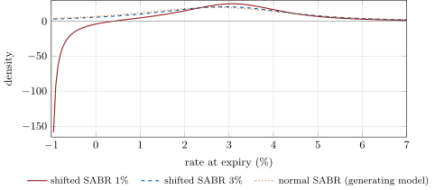
A ten-year option on a ten-year swap at 2.50%, quoted from $-200$ to $+200$ basis points around the forward (86 to 96 basis points of normal volatility), is fitted by shifted SABR with a shift of 1% (error 1.28 basis points) and of 3% (0.35). With the 1% shift the density is negative from $-0.95\%$ to $+0.35\%$ , reaching $-158$ ; with 3% it stays positive down to $-2.15\%$ (Figure 5.4). A book of low-strike receivers priced with the 1% fit carries an arbitrage against the market’s butterflies.

**Figure 5.4.** Implied densities of the ten-year into ten-year swap rate from three fits to the same quotes. The 1% shift’s density goes deeply negative just above its floor; the 3% shift’s stays positive over the range shown. Data: synthetic quotes from normal SABR; the chapter’s tutorial.

Remark 5.12 (Fixes for the wings)

Three are used: a larger shift (moving the problem below any relevant strike); solving the SABR dynamics exactly or numerically instead of expanding (the density is then positive by construction); and the free-boundary SABR of Antonov, Konikov and Spector (2015), which replaces $F^\beta$ by $|F|^\beta$ and lets the rate cross zero without a shift, with an exact price for zero correlation. Whatever the model, a density check over the strikes a book contains is a standard validation test (Chapter 26).

5.6 Tutorial: a cube from quotes

Goal. Fit a negative-rate smile with three models, calibrate and interpolate a cube, and check its density. End state: Figures 5.1, 5.3 and 5.4.

One smile: neg_fits() calibrates shifted SABR at 1% and 3% and normal SABR; deep_receiver() prices the $-0.90\%$ receiver.
The cube: build_cube() returns the calibrated sections and their errors; matrix_table() the at-the-money face.
Interpolate: missing_section(3, 7).
Density: density_table(); fig_rc_sabrcube.py writes the charts.

What to change next. Fit with $\beta=0$ and $\beta=1$ at a 3% shift and compare $\rho$ ; interpolate total variance instead of $\alpha$ along expiry and measure the error on the missing section.

5.7 Build: the swaption cube

Purpose. The volatility surface of every rates option of the book: swaptions of any expiry, tenor and strike, CMS replication (chapter 6), Bermudan calibration targets (chapters 7 to 9).

Interface. Sabr(alpha, beta, rho, nu, shift); hagan_lognormal, hagan_normal_beta0, price, normal_vol; calibrate_section(f, t, strikes, normal_vols, beta, shift, model); density; Cube(expiries, tenors, sections, forwards) with params, forward, normal_vol.

Rules. Quotes in normal volatility; $\beta$ and the shift fixed per currency; parameters interpolated, forwards taken from the curve; numpy only.

Acceptance tests. code/firm/sabrcube/tests/: the at-the-money limit of the expansion; normal SABR without vol-of-vol is Bachelier; the calibrator recovers planted parameters; payer minus receiver is the forward; a benign density is positive and integrates to one; the cube interpolates parameters bilinearly.

Stretch. Interpolation in total variance; a PDE or exact-integration SABR for positive densities; calibration to prices with bid–offer weights.

Sources and further reading

P. Hagan, D. Kumar, A. Lesniewski and D. Woodward, “Managing smile risk”, Wilmott Magazine, 2002.
A. Antonov, M. Konikov and M. Spector, “The free boundary SABR: natural extension to negative rates”, Risk, 2015.
ECB, Key ECB interest rates.
L. Andersen and V. Piterbarg, Interest Rate Modeling, volume 2, Atlantic Financial Press, 2010, chapter 16.

5.8 Exercises

Exercise 5.1 ★

A forward is $-0.30\%$ and a strike $-0.50\%$ . Can standard lognormal SABR price the option? What is the smallest shift that makes it possible?

Solution

Solution of Exercise 5.1.

No: its formula needs $F>0$ and $K>0$ (it takes $\ln(F/K)$ and powers of $FK$ ). Any shift above 0.50% makes $K+\zeta>0$ and $F+\zeta>0$ ; in practice one leaves a margin, since the density near the floor misbehaves.

Exercise 5.2 ★

In normal SABR, the forward rises by 20 basis points overnight and the parameters are unchanged. What happens to the at-the-money normal volatility, and to the volatility of the strike that was at the money yesterday?

Solution

Solution of Exercise 5.2.

The at-the-money normal volatility is unchanged ( $\alpha$ times the same factor): the backbone is flat. Yesterday’s at-the-money strike is now 20 basis points below the forward, so its volatility is the smile’s value at $F-K=+20$ basis points: the whole smile has moved with the forward.

Exercise 5.3 ★

Why do rates desks fix $\beta$ instead of fitting it?

Solution

Solution of Exercise 5.3.

Within one section $\beta$ and $\rho$ both tilt the smile and are nearly interchangeable, so a fit of both is unstable from day to day; $\beta$ is chosen for the backbone the desk believes (how the at-the-money volatility moves with the forward) and held fixed for the currency.

Exercise 5.4 ★★

With normal SABR at $\alpha=25$ basis points, $\rho=0.1$ , $\nu=0.6$ and $T=1$ , compute the at-the-money normal volatility.

Solution

Solution of Exercise 5.4.

$25\times\bigl(1+\tfrac{2-3\times0.01}{24}\times0.36\times1\bigr) = 25\times1.02955 = 25.74$ basis points, the quoted at-the-money volatility.

Exercise 5.5 ★★

In Example 5.5, why is the 1% shift fit worse at the quoted strikes as well as different in the wing?

Solution

Solution of Exercise 5.5.

The quotes were generated by a normal model; a shifted lognormal model with a small shift has a strongly level-dependent volatility, since the shifted forward $0.70\%$ is small, and its smile shape (curvature against skew) differs from the normal one, so three parameters cannot match six quotes exactly. A larger shift makes shifted SABR behave more like a normal model, and both the fit and the wing agree better.

Exercise 5.6 ★★

Read Figure 5.4. Describe the butterfly that would exploit the 1% fit near 0%, and why it is not free money in practice.

Solution

Solution of Exercise 5.6.

Buy the model’s butterfly where the density is negative (long two receivers at the middle strike, short one each at strikes a little above and below, around 0%): the model prices it negative, so a desk marking with the 1% fit would pay to sell it. In practice those strikes are not quoted, bid–offer is wide, and the market’s own prices of such butterflies are positive: the arbitrage is in the model, and a desk using it would be picked off.

Exercise 5.7 ★★★

Coding. Among shifts of 0.85%, 0.90%, 0.95% and 1%, find the smallest for which the calibrated one-year-into-two smile has a positive density from $-0.80\%$ to $+1\%$ .

Solution

Solution of Exercise 5.7.

0.90%: at 0.85% the calibrated smile’s density is negative just above the floor ( $-0.80\%$ to $-0.79\%$ ), at 0.90% it is positive from $-0.80\%$ to $+1\%$ . (Any shift must exceed 0.80% for the quoted strikes to exist at all.)

Exercise 5.8 ★★★

Find the flaw. “To fill the three-into-seven section we interpolate the quoted normal volatilities strike by strike between the neighbouring sections.” What goes wrong?

Solution

Solution of Exercise 5.8.

The sections have different forwards, so the same absolute strike sits at different moneyness in each; interpolating volatilities strike by strike mixes at-the-money and wing points, and the result need not be a SABR smile or free of arbitrage. Interpolate parameters (or moneyness-indexed volatilities), take the forward from the curve, and check the density.

5.9 Problem: The Minus-Ninety Strike

Problem 5.1

Weekend problem — a client asks for a deep receiver

In a negative-rate year a pension fund asks a desk for a receiver swaption: one year into two years, on EUR 500 million, struck at $-0.90\%$ , to protect against rates falling much further. The forward is $-0.30\%$ , the annuity 2.0, and the market quotes the six strikes of Example 5.5.

Part I — The quotes.

How far is the strike from the forward, and from the lowest quote?
Why can standard lognormal SABR not price it?
Which fits are possible, and what does each assume about the lowest rate?
Give the fit errors of the three models.
Which is the best fit at the quoted strikes?

Part II — The prices.

Give the premium in euros under each model.
By how much do the 1% and 3% shifts disagree?
Why is the 1% shift’s price the lowest?
Which price would the desk rather sell at, and which would the client rather buy at?
What is the smallest shift whose density is positive from $-0.80\%$ up?

Part III — Risk.

The desk sells at the 3% price and hedges with the quoted $-0.80\%$ receiver. What risk remains?
How does the answer change if the ECB cuts to $-0.75\%$ ?
Why is the shift itself a model parameter that needs a reserve?
What does normal SABR assume about how low rates can go?
How would you test the chosen model before quoting?

Part IV — Judgement.

Why did the euro market settle on shifts of a few per cent rather than the smallest that works?
Is a single shift for the whole cube reasonable?
What would you tell the client about the price range?
State the named result: the premium under shifts of 1% and 3%, and the smallest admissible shift.
In one sentence: what decides the price of a strike nobody quotes?

Solution

Solution of Problem 5.1.

1. 60 basis points below the forward, 10 below the lowest quote ( $-0.80\%$ ). 2. Its formula needs positive forwards and strikes. 3. Shifted SABR, which assumes the rate stays above $-\zeta$ ; normal SABR, which lets the rate take any value, with normal tails. 4. 0.77 basis points (1% shift), 0.11 (3%), zero for normal SABR (the quotes’ own model). 5. Normal SABR, then the 3% shift. 6. $0.177$ , $0.280$ and $0.295$ basis points of annuity, times $2.0\times 500$ million: EUR 17 717, 27 999 and 29 477. 7. EUR 10 282, 37% of the 3% price. 8. The modelled rate cannot go below $-1\%$ , and its volatility falls as the rate nears the floor, so the probability of finishing below $-0.90\%$ is small. 9. The desk would rather sell at the highest defensible price, the client buy at the lowest; the 1% shift is the model most favourable to the client. 10. 0.90% (exercise 7). 11. The difference between the two strikes’ dynamics: the smile slope and curvature below the quotes, i.e. the model’s wing, plus the gap between the strikes; the desk is exposed to the market re-marking the wing. 12. Rates near $-0.75\%$ would make the 1% shift’s floor almost binding and its prices meaningless; the desk would need a larger shift, and marks would jump when it changed. 13. Its choice moves the prices of unquoted strikes by tens of per cent (here 37%) while fitting quoted strikes equally well; that is model uncertainty, and a reserve covers the spread of prices across admissible shifts. 14. Nothing: the rate is normal given the volatility, unbounded below, which puts more weight on very negative rates than any shifted model. 15. Fit all candidate models; check densities over the book’s strikes; compare wing prices across models and with any traded points (dealer polls); backtest the smile’s behaviour when the forward moved. 16. To keep the floor well below any plausible rate, so that the wing of the distribution, and the prices of low strikes, do not depend on where the floor is; a small shift makes the smile hostage to it. 17. Reasonable within a currency if it is well below the effective lower bound; the choice is part of the market convention, which makes quotes comparable. 18. That quoted strikes pin the price only near the forward, that three standard models give EUR 17 700 to 29 500, and what the desk charges and why. 19. Named result: the minus-ninety strike costs EUR 17 717 with a 1% shift and EUR 27 999 with 3% (37% apart), and 0.90% is the smallest shift that keeps the density positive from $-0.80\%$ up. 20. The model’s assumption about how low rates can go and how volatile they are near that bound.

5.10 Interview questions

Interview question 5.1 ★ trader, researcher

How did the rates market price options when rates went negative?

Solution

Solution of Interview question 5.1.

By leaving lognormal (Black) quotes, which cannot represent negative forwards or strikes: quoting normal (Bachelier) volatilities, or Black volatilities of a shifted rate $F+\zeta$ ; models moved to normal SABR or shifted SABR, later also free-boundary SABR.

What the interviewer is looking for: normal quotes and shifted models, and why Black fails.

Interview question 5.2 ★★ researcher

What does $\beta$ control in SABR, and why is it usually fixed?

Solution

Solution of Interview question 5.2.

$\beta$ sets the backbone: how the at-the-money volatility moves with the forward ( $\beta=0$ flat in normal terms, $\beta=1$ flat in lognormal terms) and part of the skew. Since $\rho$ also sets the skew, fitting both on one smile is unstable; $\beta$ is fixed from the desk’s view of the backbone or a historical regression of at-the-money volatility on the forward.

What the interviewer is looking for: backbone versus skew, and the identification problem.

Interview question 5.3 ★★ researcher, developer

How would you build a swaption cube from broker quotes?

Solution

Solution of Interview question 5.3.

For each (expiry, tenor): forward and annuity from the multi-curve; clean the quotes (normal vols or premiums, straddles and strangles); fix $\beta$ and the shift; fit $\alpha,\rho,\nu$ with bounds; check errors and parameter smoothness across the grid; interpolate parameters (variance in expiry); check density and calendar arbitrage; publish with diagnostics.

What the interviewer is looking for: a pipeline with checks, not only a fit.

Interview question 5.4 ★★ trader

The forward moves up ten basis points. What happens to the smile under normal SABR and under lognormal SABR with $\beta=1$ ?

Solution

Solution of Interview question 5.4.

Normal SABR: the smile shifts right by ten basis points, the at-the-money normal volatility unchanged. Lognormal with $\beta=1$ : the at-the-money Black volatility is unchanged, so the normal volatility rises roughly in proportion to the forward, and the smile moves in relative (log-moneyness) terms.

What the interviewer is looking for: the two backbones.

Interview question 5.5 ★★★ researcher, risk

Hagan’s formula gives a negative density. Where, why, and what do you do?

Solution

Solution of Interview question 5.5.

In the low-strike wing of long expiries (large $\nu^2T$ ), near the lower bound of the rate, because the expansion is asymptotic and misrepresents the absorbing boundary. Fixes: a larger shift, an exact or numerical SABR (PDE, integration), free-boundary SABR, or wing extrapolation with a positive density; always test the density over the book’s strikes.

What the interviewer is looking for: the cause and the fixes.

Interview question 5.6 ★★★ developer

Your cube calibration fails on one section every morning. How do you investigate?

Solution

Solution of Interview question 5.6.

Look at the inputs first: stale or crossed quotes, a forward from the wrong curve, a strike grid shifted by the forward; then at the fit: starting point, bounds hit ( $\rho$ near $\pm1$ , $\nu$ exploding), conversion failures of deep quotes to the model’s volatility; compare with yesterday’s parameters and the neighbouring sections; add a regularisation towards neighbours if the section is thinly quoted.

What the interviewer is looking for: data before optimiser, and a systematic check.

Terms defined in this chapter

See all 2333 terms in the glossary