Rates, Credit, XVA and Risk · Rates, credit & risk

23Regulatory Capital for Trading Books

Under the market-risk rules that the Basel Committee finalised in January 2019, a bank that wants to set a desk’s capital with its own model must show, every quarter, that the model explains the desk’s own P&L. If the risk model’s P&L and the P&L of the pricing systems diverge too much, the desk pays a surcharge; if they diverge further, the desk loses the model and falls back on a standardised formula that, for the book of this chapter, is almost three times as high. The rules took years to reach the statute books: deferred once by the Committee, postponed for two years in the European Union, delayed in the United Kingdom, and still a proposal in the United States in 2026. This chapter computes both approaches on chapter 21’s book: the standardised sensitivities, the expected shortfall with its stressed calibration, and the attribution test that decides between them.

23.1 The trading book and its boundary

Definition 23.1 (Fundamental Review of the Trading Book)

The Fundamental Review of the Trading Book (FRTB) is the Basel Committee’s market-risk capital framework of January 2019: a revised boundary between the books, a standardised approach built on sensitivities, and an internal models approach built on expected shortfall with desk-level eligibility tests.

Definition 23.2 (Trading book, banking book)

The trading book holds instruments held for short-term resale, for profiting from short-term price movements, for locking in arbitrage profits, or for hedging such positions, fair valued daily through P&L; everything else is in the banking book, whose market risk (mainly interest rates) is managed as in chapter 24.

The boundary matters because the two books carry different capital; moving instruments between them to reduce capital is restricted and, where allowed, any capital benefit is disallowed.

23.2 The standardised approach: sensitivities, curvature, default and residual risks

Definition 23.3 (Sensitivities-based method)

The sensitivities-based method computes prescribed sensitivities (a PV01 per tenor for interest rates, the value change for a 1% move for FX), multiplies them by prescribed risk weights, and aggregates the weighted sensitivities within buckets ( $K_b = \sqrt{\max(0,\sum_{kl}\rho_{kl}WS_kWS_l)}$ ) and across buckets ( $\sqrt{\sum_bK_b^2+\sum_{b\ne c}\gamma_{bc}S_bS_c}$ ), under three correlation scenarios (the prescribed correlations, 1.25 times them capped at one, and $\max(2\rho-1,0.75\rho)$ ); the requirement is the largest of the three totals.

Definition 23.4 (Curvature risk charge)

The curvature risk charge captures the losses of options beyond their delta: each risk factor is shocked up and down by its risk weight, and the loss beyond the delta term, $\mathrm{CVR}^\pm = -\sum_i(V_i(x^\pm)-V_i(x)\mp\mathrm{RW}\,s_i)$ , is charged, the larger of the two directions.

Definition 23.5 (Default risk charge, residual risk add-on)

The default risk charge captures the jump-to-default risk of credit and equity positions that spread shocks miss. The residual risk add-on charges a flat share of notional for risks the sensitivities do not capture: 1% for instruments with exotic underlyings, 0.1% for other residual risks.

def within(ws: np.ndarray, corr: np.ndarray) -> float:
    return math.sqrt(max(0.0, float(ws @ corr @ ws)))


def across(K: Sequence[float], S: Sequence[float], gamma: float) -> float:
    K, S = np.asarray(K, float), np.asarray(S, float)
    n = len(K)

    def total(s):
        return float((K ** 2).sum() + sum(gamma * s[b] * s[c] for b in range(n) for c in range(n) if b != c))

    t = total(S)
    if t < 0:
        t = total(np.clip(S, -K, K))
    return math.sqrt(max(t, 0.0))


def girr_delta(sens: dict[str, dict[float, float]], which: str = "medium", specified: bool = True) -> float:
    """sens: currency -> {tenor: PV01 / 0.0001 (value change per unit rate)}."""
    Ks, Ss = [], []
    for ccy in sens:
        tenors = sorted(sens[ccy])
        ws = np.array([GIRR_RW[t] / (math.sqrt(2) if specified else 1.0) * sens[ccy][t] for t in tenors])
        corr = np.array([[1.0 if a == b else scenario(girr_rho(a, b), which) for b in tenors] for a in tenors])
        Ks.append(within(ws, corr))
        Ss.append(float(ws.sum()))
    return across(Ks, Ss, scenario(GIRR_GAMMA, which))

Listing 23.1. Within- and across-bucket aggregation, and the GIRR delta charge under a correlation scenario. code/firm/frtb/firm_frtb.py

Example 23.6 (The standardised charge of the book)

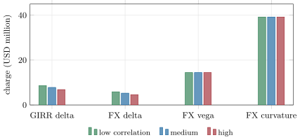
Chapter 21’s book, on 23 September 2026. Its GIRR sensitivities (mapping the two bonds’ par-yield sensitivities to the two- and ten-year USD tenors, a simplification) are $+56\,525$ and $-155\,012$ dollars per basis point; with risk weights $1.3\%/\sqrt2$ and $1.1\%/\sqrt2$ and a correlation of 88.7%, the GIRR delta charge is USD 7.83 million. FX delta (EUR and JPY, risk weight $15\%/\sqrt2$ , cross-currency correlation 60%) is USD 5.30 million; FX vega, the straddle’s vega times its 8% volatility at a 100% risk weight, USD 14.49 million; FX curvature, from shocking EURUSD by $\pm10.6\%$ , USD 39.23 million. In the low correlation scenario the total is USD 68.29 million, the largest of the three (Figure 23.1).

**Figure 23.1.** Standardised charges of chapter 21’s book by component and correlation scenario. The short straddle’s curvature dominates; the delta charges move with the scenario (lower correlations remove the offset between the two- and ten-year positions), vega and a single curvature factor do not. Data: the chapter’s tutorial.

23.3 The internal models approach: expected shortfall with liquidity horizons

Definition 23.7 (Internal models approach, liquidity horizon)

The internal models approach sets capital from the bank’s own model of expected shortfall at 97.5%, computed on a ten-day base horizon and scaled up for risk factors with longer liquidity horizons (10, 20, 40, 60 or 120 days, the time assumed to exit or hedge a position without moving prices): $\mathrm{ES} = \sqrt{\mathrm{ES}_T(P)^2+\sum_{j\ge2}\bigl(\mathrm{ES}_T(P,j)\sqrt{(\mathrm{LH}_j-\mathrm{LH}_{j-1})/T}\bigr)^2}$ .

Definition 23.8 (Stressed expected shortfall)

Stressed expected shortfall calibrates the ES to the most severe twelve-month period for the bank’s portfolio, computed on a reduced set of risk factors with a long history and scaled up by the ratio of the current ES with all factors to the current ES with the reduced set (at least one).

The idea is older than the FRTB: the Basel Committee’s July 2009 revisions (Basel 2.5) added to the VaR charge a stressed VaR, a ten-day 99% VaR of the current portfolio calibrated to a continuous twelve-month period of significant stress, such as 2007–08, each charge taken as the higher of its latest value and a multiple of its sixty-day average.

Capital for modellable factors is $\mathrm{IMCC} = \rho\,\mathrm{ES}(\text{all})+(1-\rho)\sum_i\mathrm{ES}(\text{class }i)$ with $\rho = 0.5$ , half the diversified ES and half the sum over risk classes, and the requirement is the larger of yesterday’s IMCC and 1.5 times its sixty-day average, plus the stressed charge for non-modellable factors.

Example 23.9 (The internal-model charge)

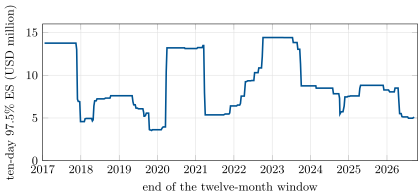
On overlapping ten-day moves, the book’s 97.5% ES over the last year is USD 5.27 million. Scanning every twelve-month window since 2016, the most severe ends on 3 October 2022 (Figure 23.2): its ES is USD 14.41 million for the whole book, 5.67 million for rates alone and 14.01 million for FX alone. All the factors are major-currency rates and FX pairs with a ten-day liquidity horizon, so no scaling applies. The IMCC is $0.5\times14.41+0.5\times(5.67+14.01) = \text{USD}~17.04$ million and, with the multiplier of 1.5, the charge is USD 25.56 million, 37% of the standardised one.

**Figure 23.2.** Expected shortfall of today’s book over every twelve-month window of history since 2016, by the window’s end date. The stressed calibration takes the maximum, the year to October 2022. Data: US Treasury par yields, ECB reference rates; the chapter’s tutorial.

23.4 Backtesting and the P&L attribution test

Definition 23.10 (Hypothetical and risk-theoretical P&L)

The hypothetical P&L (HPL) of a desk is the daily change in the value of yesterday’s positions computed by the bank’s pricing systems with today’s market data. The risk-theoretical P&L (RTPL) is the same change computed by the risk model, from its own risk factors and its own revaluation.

Definition 23.11 (P&L attribution test)

The P&L attribution test compares a desk’s HPL and RTPL over 250 days by the Spearman correlation of their ranks and the Kolmogorov–Smirnov distance between their distributions: green if the correlation exceeds 0.80 and the distance is below 0.09, red if the correlation is below 0.70 or the distance above 0.12, amber otherwise. Red desks use the standardised approach; amber desks pay a surcharge of half the gap between the standardised and internal-model charges (for a bank whose only desk is amber).

def _ranks(x: np.ndarray) -> np.ndarray:
    order = np.argsort(x, kind="mergesort")
    r = np.empty(len(x))
    r[order] = np.arange(len(x))
    return r


def spearman(a: np.ndarray, b: np.ndarray) -> float:
    return float(np.corrcoef(_ranks(np.asarray(a)), _ranks(np.asarray(b)))[0, 1])


def ks_stat(a: np.ndarray, b: np.ndarray) -> float:
    grid = np.sort(np.concatenate([a, b]))
    fa = np.searchsorted(np.sort(a), grid, side="right") / len(a)
    fb = np.searchsorted(np.sort(b), grid, side="right") / len(b)
    return float(np.max(np.abs(fa - fb)))


def pla_zone(sp: float, ks: float) -> str:
    if sp > 0.80 and ks < 0.09:
        return "green"
    if sp < 0.70 or ks > 0.12:
        return "red"
    return "amber"

Listing 23.2. Spearman’s rank correlation, the Kolmogorov–Smirnov distance and the attribution zones. code/firm/frtb/firm_frtb.py

Example 23.12 (Three risk models of the same desk)

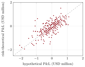
Over the last 250 days, a risk model that revalues the book with the delta–gamma expansion passes easily (Spearman 1.00, KS 0.008). One that has no yen factor passes too (0.956 and 0.060). One that has no two-year factor is amber through its distribution (0.949 and 0.100). One that proxies the ten-year yield by the two-year, a common response to a factor judged non-modellable, is amber through its correlation: 0.703 and 0.044 (Figure 23.3).

**Figure 23.3.** Daily hypothetical P&L of the book against the P&L of a risk model that proxies the ten-year yield by the two-year, over 250 days. The ranks agree only loosely (Spearman 0.703): amber. Data: US Treasury, ECB; the chapter’s tutorial.

23.5 Non-modellable risk factors

Definition 23.13 (Risk-factor eligibility test, non-modellable risk factor)

The risk-factor eligibility test admits a risk factor into the internal model if it has at least 24 real price observations in the past year with no 90-day period holding fewer than four (or at least 100 in the year). A factor that fails is a non-modellable risk factor: it is capitalised separately by its own stress scenario, with little diversification.

As of September 2026 — When the FRTB applies

The Basel Committee’s January 2019 standard was to apply from 1 January 2022; in March 2020 its oversight body deferred it to 1 January 2023. In the European Union, after the rules were postponed by two years, they apply from 1 January 2027 with targeted, temporary adjustments for three years, including a capital multiplier (Commission delegated act adopted on 4 June 2026, published on 1 September 2026). In the United Kingdom, the PRA consulted in June 2026 on its internal model rules, to apply from 1 January 2028 with the attribution test’s monitoring period extended from one to three years; its other Basel 3.1 rules apply from January 2027. In the United States, the agencies proposed in March 2026 a framework implementing the final Basel III components, with market-risk rules for banks with significant trading activity; comments closed on 18 June 2026.

23.6 Tutorial: two capital numbers for one desk

Goal. Compute the standardised and internal-model charges of chapter 21’s book and run the attribution test on several risk models. End state: the numbers of Examples 23.6, 23.9 and 23.12 and the three charts.

Sensitivities: sensitivities() bumps the book as the standard prescribes.
Standardised: standardised() under the three scenarios.
Internal models: internal_models() with the stressed window.
Attribution: pla(variant); fig_rc_frtb.py writes the charts.

What to change next. Halve the straddle and see which charge moves most; give the yen a twenty-day liquidity horizon and apply the scaling formula.

23.7 Build: the FRTB engine

Purpose. The firm’s market-risk capital under both approaches and its desk eligibility tests, fed by the risk engine of chapter 29.

Interface. girr_rho, scenario, within, across; girr_delta, fx_delta, fx_vega, cvr, fx_curvature, sbm; es, es_liquidity, imcc, ima_capital, amber_surcharge; spearman, ks_stat, pla_zone; rfet.

Rules. Parameters as in the Basel standard of January 2019; GIRR and FX risk classes only; specified currencies with the $\sqrt2$ reduction; the largest scenario total.

Acceptance tests. code/firm/frtb/tests/: the standard’s correlation example (88.69%); scenario transforms; aggregation with its fallback; curvature signs; capital formula and surcharge; liquidity scaling; attribution statistics and zone boundaries; eligibility test.

Stretch. Credit spread, equity and commodity classes; the default risk charge; the residual risk add-on; non-modellable stress scenarios; national variations (EU multipliers).

Sources and further reading

Basel Committee on Banking Supervision, Minimum capital requirements for market risk, January 2019.
Bank for International Settlements, press release of 27 March 2020 on the deferral of Basel III.
European Commission, “Commission adopts temporary adjustments to Basel III market risk rules”, 4 June 2026.
Bank of England, “PRA sets out adjustments to its market risk internal model approach under Basel 3.1”, 19 June 2026.
Board of Governors of the Federal Reserve System, press release of 19 March 2026 on proposals to modernise the regulatory capital framework.

23.8 Exercises

Exercise 23.1 ★

Compute the GIRR correlation between the two- and ten-year tenors and its high and low scenario values.

Solution

Solution of Exercise 23.1.

$\max(e^{-0.03\times8/2},0.40) = e^{-0.12} = 88.7\%$ ; high $\min(1.25\times0.887,1) = 100\%$ ; low $\max(2\times0.887-1,0.75\times0.887) = 77.4\%$ .

Exercise 23.2 ★

Why did the low correlation scenario give the largest total for this book?

Solution

Solution of Exercise 23.2.

The book is long the ten-year and short the two-year: the positions offset through their positive correlation, and less correlation means less offset. The same happens across the long-euro and short-yen FX buckets. With the vega and curvature charges unchanged, the low scenario adds most.

Exercise 23.3 ★

A desk’s attribution statistics are 0.82 and 0.10. What zone is it in, and what happens?

Solution

Solution of Exercise 23.3.

Amber: the correlation passes (above 0.80) but the distribution distance (0.10) lies between 0.09 and 0.12. The desk keeps the internal model but pays the surcharge.

Exercise 23.4 ★★

Why is the internal-model charge so much lower than the standardised one for this book?

Solution

Solution of Exercise 23.4.

The standardised approach charges the straddle’s curvature (a $\pm10.6\%$ EURUSD shock) and its vega at a 100% weight, sizes calibrated for any bank’s book; the internal model measures the ten-day ES of the actual book, where EURUSD moves are far smaller, even in the stressed year, and diversification applies.

Exercise 23.5 ★★

A risk factor has 30 observations in the year, all in its first four months. Is it modellable?

Solution

Solution of Exercise 23.5.

No: it has more than 24 observations, but the last eight months include 90-day periods with none, so criterion (1) fails, and 30 is below the 100 of criterion (2). It is non-modellable.

Exercise 23.6 ★★

Why does the IMCC mix the diversified ES with the sum of risk-class ES?

Solution

Solution of Exercise 23.6.

The diversified ES relies on the model’s cross-class correlations, which can break in stress; the sum over classes assumes none. Weighting them half and half limits the capital benefit of cross-class diversification.

Exercise 23.7 ★★★

Coding. Compute the ES of a portfolio whose risk factors split into a ten-day group with ES 5 and a twenty-day group with ES 3 (where the second is also counted in the first), using the liquidity-horizon formula.

Solution

Solution of Exercise 23.7.

$\sqrt{5^2+\bigl(3\sqrt{(20-10)/10}\bigr)^2} = \sqrt{34} = 5.83$ .

Exercise 23.8 ★★★

Find the flaw. “Our internal model gives a third of the standardised capital; the model is better, so the regulator should let us use it for every desk.”

Solution

Solution of Exercise 23.8.

Lower is not better: the model must pass backtesting and attribution desk by desk, its stressed calibration and non-modellable factors add capital, and the standardised approach remains a benchmark (and in some jurisdictions a floor). A low number with a failing attribution test is evidence against the model.

23.9 Problem: The Desk That Failed Attribution

Problem 23.1

Weekend problem — amber

Chapter 21’s book is the only desk of a bank using the internal models approach. Its risk model has no reliable ten-year data and proxies the ten-year yield by the two-year.

Part I — Two numbers.

Give the standardised charge and the scenario that sets it.
Give the internal-model charge and its ingredients.
Which component drives the standardised charge?
Why is the stressed window the year to October 2022 for this book?
What would a longer FX volatility liquidity horizon change?

Part II — The test.

Give the Spearman correlation and KS distance of the proxy model.
Give the zone and why.
Give the surcharge and the resulting capital.
What would red mean for the desk’s capital?
Which of the other risk models would pass, and which fail?

Part III — Fixing it.

Why does the proxy fail the rank correlation but not the distribution test?
What data would make the ten-year yield modellable?
Would a better proxy (a regression on the two-year) help?
What does a desk gain from a longer monitoring period, as the PRA proposes?
How should the desk’s business decide between the fix and the surcharge?

Part IV — Judgement.

Why test attribution at all when backtesting exists?
What incentives does the amber surcharge create?
How do the EU multipliers and the UK delay change a global bank’s choices?
State the named result: the desk’s internal-model and standardised capital, and the Spearman and KS values that put it in amber.
In one sentence: what does the attribution test really check?

Solution

Solution of Problem 23.1.

1. USD 68.29 million, in the low correlation scenario. 2. USD 25.56 million: 1.5 times an IMCC of 17.04 million, from a stressed ES of 14.41 million for the book and 5.67 and 14.01 million for rates and FX. 3. FX curvature, USD 39.23 million, from the short straddle. 4. It contains the dollar’s surge and the euro’s fall below parity, the largest EURUSD moves in the sample, which the short straddle and the euro position feel most. 5. Nothing in the internal model here, since volatility is not a modelled factor; in a model with it, a 40-day horizon would scale up the vega-driven ES. 6. 0.703 and 0.044. 7. Amber: the correlation is between 0.70 and 0.80; the distance passes. 8. A surcharge of $0.5\times(68.29-25.56) = \text{USD}~21.36$ million; capital USD 46.93 million. 9. The standardised charge, USD 68.29 million. 10. The delta–gamma and no-yen models pass (green); the no-two-year model is amber through its distance (0.100). 11. The proxy moves the two tenors together, so it misses the days the curve twists: the order of the daily P&Ls (ranks) is scrambled, while the spread of the distribution stays similar. 12. Real price observations of ten-year swaps or bonds: at least 24 a year with no 90-day gap holding fewer than four. 13. Partly: a regression scales the move but still cannot see the twist; only a separate factor restores the ranks. 14. Time to gather data and fix the model before the test affects capital. 15. Compare the fix’s cost with the surcharge’s present value over the desk’s horizon, and the risk of falling to red. 16. Backtesting checks the tail count; attribution checks that the risk model sees the same P&L drivers every day. A model can pass one and fail the other. 17. To improve risk models, or to game the statistics by choosing proxies that preserve ranks. 18. Where the rules and multipliers differ, a bank may book trades in the jurisdiction with the lighter treatment, or run different models. 19. Named result: the desk that failed attribution: internal-model capital USD 25.56 million, standardised USD 68.29 million; Spearman 0.703 and KS 0.044 put it in amber, and capital becomes USD 46.93 million. 20. That the risk model and the pricing systems see the same world.

23.10 Interview questions

Interview question 23.1 ★ risk, bank

What changed from Basel 2.5 to the FRTB?

Solution

Solution of Interview question 23.1.

VaR and stressed VaR at 99% replaced by expected shortfall at 97.5% with liquidity horizons and stressed calibration; a sensitivity-based standardised approach; desk-level approval with backtesting and P&L attribution; non-modellable risk factors; a stricter book boundary.

What the interviewer is looking for: ES, liquidity horizons, SBM and desk-level tests.

Interview question 23.2 ★★ risk, developer

Walk through the sensitivities-based method for an interest rate swap book.

Solution

Solution of Interview question 23.2.

PV01 by currency and tenor; risk weights per tenor (divided by $\sqrt2$ for major currencies); aggregation within the currency with tenor correlations and across currencies at 50%; the three correlation scenarios; curvature from parallel shocks if there are options.

What the interviewer is looking for: the steps and parameters.

Interview question 23.3 ★★ risk

What is the P&L attribution test and why do desks fail it?

Solution

Solution of Interview question 23.3.

It compares the risk model’s P&L with the front office’s by rank correlation and a distribution distance. Desks fail from missing or proxied risk factors, different data sources or snapshot times, simplified revaluation, and basis risks.

What the interviewer is looking for: the metrics and the common causes.

Interview question 23.4 ★★ researcher, risk

Why expected shortfall with liquidity horizons rather than a ten-day VaR?

Solution

Solution of Interview question 23.4.

ES sees the size of tail losses and is coherent; liquidity horizons reflect that some positions take weeks to exit, which a uniform ten-day VaR ignores; stressed calibration avoids capital falling in calm markets.

What the interviewer is looking for: tail, liquidity and procyclicality.

Interview question 23.5 ★★★ bank

How would you decide which desks should apply for internal-model approval?

Solution

Solution of Interview question 23.5.

By the capital saving against the cost of models, data and controls, and by the likelihood of passing backtesting, attribution and eligibility tests; desks with liquid, well-modelled risks first.

What the interviewer is looking for: cost-benefit and test risk.

Interview question 23.6 ★★★ developer

What data and systems does a bank need to run the internal models approach?

Solution

Solution of Interview question 23.6.

Long histories of real prices per risk factor with observation counts; consistent market data for front office and risk; daily HPL and RTPL by desk; full revaluation infrastructure for ES over many scenarios and liquidity subsets; stress-period search; reporting and audit trails.

What the interviewer is looking for: data, revaluation and controls.

Terms defined in this chapter

See all 2333 terms in the glossary