Rates, Credit, XVA and Risk · Rates, credit & risk

3Rates Risk

A dollar swap desk holds two hundred swaps, USD 12 billion of notional, and its risk report shows a parallel DV01 of zero: a one-basis-point rise of every rate would leave it exactly where it is. Replay on it the moves of the US Treasury curve on 21 October 2022, when the two-year yield fell 13 basis points and the thirty-year rose 9, and it loses three million dollars. The report was right about the level and silent about the shape. Rates risk is a vector, one number per point of the curve, and managing it means choosing the coordinates in which to read the vector, knowing how the curve actually moves, and hedging with a handful of instruments a risk spread over many. This chapter does all three on chapter 1’s curve builder, with ten years of daily Treasury data as the model of how curves move.

3.1 Bucketed sensitivities and risk ladders

Definition 3.1 (Bucketed sensitivity, risk ladder)

A bucketed sensitivity $\Delta_k$ of a position is the change in its value when the $k$ -th input quote of the curve rises by one basis point and the curve is recalibrated, the others held. The risk ladder is the vector $(\Delta_1,\dots,\Delta_n)$ over all inputs; its sum is the sensitivity to a parallel shift of the quotes, and its dot product with a vector of quote moves $\delta q$ (in basis points) is the first-order P&L, $\pnl\approx\sum_k\Delta_k\,\delta q_k$ .

A par swap maturing on a pillar loads only that pillar under a local interpolation (Proposition 1.3): on the chapter’s eight-pillar curve (flat forwards, par SOFR swaps at 1, 2, 3, 5, 7, 10, 20 and 30 years) a ten-year payer of USD 100 million has a ladder of USD 83 778 on the ten-year quote and zero elsewhere. A book’s ladder is the sum of its trades’.

Example 3.2 (The desk’s ladder)

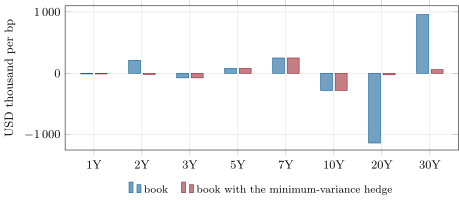
The chapter’s book holds 200 swaps of random maturity, direction and size (seeded), plus a two-year payer of USD 1.471 billion and a thirty-year payer of USD 281 million added so that the parallel DV01 is zero. Its ladder (Figure 3.1) is anything but zero: $+212\,010$ at two years, $+249\,817$ at seven, $-279\,791$ at ten, $-1\,135\,816$ at twenty and $+958\,308$ at thirty, per basis point.

The risk ladder of the chapter’s 200-swap book, whose buckets sum to zero, and the ladder after the three-swap hedge of (two-, twenty- and thirty-year swaps). The hedge does not zero those three buckets; it leaves the combination of risks that historical moves make cheapest to carry. Data: the chapter’s illustrative book and tutorial. — **Figure 3.1.** The risk ladder of the chapter’s 200-swap book, whose buckets sum to zero, and the ladder after the three-swap hedge of Example 3.11 (two-, twenty- and thirty-year swaps). The hedge does not zero those three buckets; it leaves the combination of risks that historical moves make cheapest to carry. Data: the chapter’s illustrative book and tutorial.

3.2 From par risk to zero risk: the Jacobian

The ladder above is in the coordinates of the input quotes. Models, scenario engines and regulators often want it in other coordinates: zero rates at the pillars, forward rates, or a standard set of key maturities.

Definition 3.3 (Curve Jacobian)

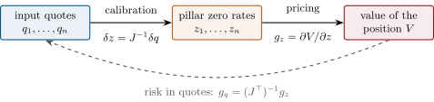
The curve Jacobian is the matrix $J_{kj} = \partial m_k/\partial z_j$ of the derivatives of the model quotes of the input instruments with respect to the curve’s pillar parameters, at the calibrated curve; its inverse gives how the pillars move when the quotes move, $\delta z = J^{-1}\delta q$ .

Proposition 3.4 (Changing coordinates)

Let $g_q = (\partial V/\partial q_k)_k$ and $g_z = (\partial V/\partial z_j)_j$ be the ladders of a position in quotes and in pillar zero rates. Then

g_z = J^\top g_q,\qquad g_q = (J^\top)^{-1}g_z .

Proof. The position depends on the quotes only through the pillars, $V = V(z(q))$ , so $g_q = (\partial z/\partial q)^\top g_z = (J^{-1})^\top g_z$ . ∎

Two coordinate systems for one risk. Calibration maps quotes to pillars, pricing maps pillars to value; the Jacobian of the calibration carries a ladder from one system to the other (). — **Figure 3.2.** Two coordinate systems for one risk. Calibration maps quotes to pillars, pricing maps pillars to value; the Jacobian of the calibration carries a ladder from one system to the other (Proposition 3.4).

Example 3.5 (Two ladders of one swap)

The ten-year payer’s par ladder is $83\,778$ on the ten-year quote alone; its zero ladder is $367$ , $713$ , $1\,531$ , $3\,205$ , $5\,120$ and $74\,016$ on the one- to ten-year pillars. Raising an early zero rate lowers the value of the fixed coupons the payer owes, and in quote space that effect is absorbed by recalibration. For the whole book, the par ladder sums to zero and the zero ladder to USD 11 408: a parallel shift of quotes and a parallel shift of zero rates are different scenarios.

Definition 3.6 (Key-rate duration)

A key-rate duration (Ho, 1992) is the sensitivity of a position to a “tent” shift of the zero curve centred on one key maturity: one basis point at the key, falling linearly to zero at the two neighbouring keys. The tents sum to one at every maturity, so key-rate sensitivities add up to the sensitivity to a parallel shift of zero rates; they are independent of how the curve was built, which makes them the usual currency of risk reports across desks.

3.3 Principal components of the curve

How do curves move? The covariance matrix of daily changes answers, and its eigenvectors, the principal components of One Quant Book 4, chapter 22, give the answer a shape.

Definition 3.7 (Level, slope and curvature factors)

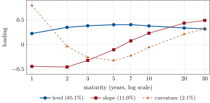
For a curve sampled at $n$ maturities, let $v_1, v_2, v_3$ be the first three eigenvectors of the covariance of its daily changes (with $\lambda_1\ge \lambda_2\ge\lambda_3$ ). The level factor $v_1$ has loadings of one sign, the slope factor $v_2$ changes sign once, from short to long maturities, and the curvature factor $v_3$ changes sign twice. The move of day $t$ has score $v_i^\top\delta q_t$ on factor $i$ , and the factors are uncorrelated by construction.

Example 3.8 (Ten years of Treasury moves)

Over the 2 681 daily changes of the US Treasury par curve from January 2016 to September 2026 (eight maturities from one to thirty years), the first three components explain 85.1%, 11.0% and 2.1% of the variance, 98.2% together, with daily standard deviations of 13.6, 4.9 and 2.1 basis points of score (Figure 3.3). The level loads less on the one-year than on the belly; the curvature factor is dominated by the one-year yield, the maturity most tied to the next policy meetings. Litterman and Scheinkman found the same three factors in 1991.

**Figure 3.3.** Loadings of the first three principal components of daily changes of US Treasury par yields, January 2016 to September 2026, with their shares of variance. Source: US Treasury, daily par yield curve rates (public domain); the chapter’s tutorial.

Remark 3.9 (The loss of the hook, factor by factor)

Decomposing the move of 21 October 2022 and the book’s ladder on all eight components, the slope factor (score $+21.2$ ) accounts for $-\text{USD}~3.09$ million of the $-3.00$ million first-order loss, and the higher components add $+0.72$ , $+0.69$ and $-1.48$ million that nearly cancel. The book was level-neutral and short a steepening.

3.4 Hedging a swap book

A book’s ladder has as many buckets as the curve has pillars; a desk hedges it with a few liquid swaps. Which ones, and how much of each, depends on how the buckets move together.

Method 3.10 (Minimum-variance hedge)

Let $g$ be the book’s ladder, $H$ the matrix whose columns are the ladders of one unit of each hedge instrument, and $\Sigma$ the covariance of daily quote moves. The daily P&L of book plus hedge is $(g+Hh)^\top\delta q$ , of variance $(g+Hh)^\top\Sigma(g+Hh)$ , minimised by

h^\star = -\bigl(H^\top\Sigma H\bigr)^{-1}H^\top\Sigma g .

Report the residual share of variance $(g+Hh^\star)^\top\Sigma(g+Hh^\star) / g^\top\Sigma g$ , and choose the instruments that make it smallest.

def min_variance_hedge(g: np.ndarray, hedges: np.ndarray, cov: np.ndarray) -> tuple[np.ndarray, float]:
    """Quantities h of the hedge instruments (columns of `hedges` are their ladders) minimising the
    variance of (g + hedges h) . dq under covariance `cov` of the moves dq. Returns h and the share
    of the book's variance that remains."""
    a = hedges.T @ cov @ hedges
    h = -np.linalg.solve(a, hedges.T @ cov @ g)
    resid = g + hedges @ h
    return h, float(resid @ cov @ resid / (g @ cov @ g))

Listing 3.1. The minimum-variance hedge and the variance it leaves. code/firm/ratesrisk/firm_ratesrisk.py

Example 3.11 (Three swaps against two hundred)

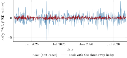
With Treasury par-yield changes standing in for swap-rate changes, the book’s daily P&L has a standard deviation of USD 1 288 843. The textbook trio of two-, ten- and thirty-year swaps leaves 58.3% of the variance; hedging the three principal components exactly leaves 68.9%, because most of the book’s risk lies in the twenty-against-thirty-year spread, which the first three factors do not describe. The best three swaps are the two-, twenty- and thirty-year: receive fixed on USD 1.196 billion of two-year, pay on USD 801 million of twenty-year and receive on USD 515 million of thirty-year. They leave 4.2% of the variance, a daily standard deviation of USD 264 554 (Figure 3.4).

First-order daily P&L of the book, g q_t, on the Treasury par-yield moves of September 2024 to September 2026, unhedged and with the minimum-variance two-, twenty- and thirty-year hedge (estimated on 2016–2026). Source: US Treasury par yields; the chapter’s tutorial. — **Figure 3.4.** First-order daily P&L of the book, $g^\top\delta q_t$ , on the Treasury par-yield moves of September 2024 to September 2026, unhedged and with the minimum-variance two-, twenty- and thirty-year hedge (estimated on 2016–2026). Source: US Treasury par yields; the chapter’s tutorial.

Remark 3.12 (What the hedge assumes)

The hedge is only as good as its covariance: ten years of Treasury moves include the zero-rate years and the 2022 hikes, and swap rates move with Treasury yields plus swap spreads, which this model ignores. A hedge estimated on one regime and run in another leaves more than 4%; stress tests (Chapter 22) exist for that.

3.5 Gamma and cross-gamma

The ladder is a first derivative; for large moves the second derivatives matter.

Definition 3.13 (Cross-gamma)

The cross-gamma of a position between inputs $k$ and $l$ is $\Gamma_{kl} = \partial^2V/\partial q_k\partial q_l$ for $k\ne l$ , per square basis point; with the diagonal terms it forms the gamma matrix, and the second-order P&L is $\sum_k\Delta_k\delta q_k + \tfrac12\sum_{k,l}\Gamma_{kl}\delta q_k\delta q_l$ .

Example 3.14 (The second-order term of the hook)

On the move of 21 October 2022 the book’s ladder gives a first-order loss of exactly USD 3 000 000 (by construction); full revaluation gives $-3\,077\,970$ . The gamma matrix, computed by central differences, gives $\tfrac12\,\delta q^\top\Gamma\,\delta q = -78\,189$ , which accounts for the difference to within USD 220. The book’s parallel gamma is $-377$ dollars per square basis point: it is short convexity, mostly through its thirty-year payers.

For a swap book cross-gamma is small and mostly comes from discounting; for options, and for products whose payoff depends on two rates (chapter 6), it is first order.

3.6 Tutorial: ladder, factors and hedge

Goal. Measure the book’s risk in quote, zero and key-rate coordinates, find how the Treasury curve moves, and hedge the book with three swaps. End state: Figures 3.1, 3.3 and 3.4 and the numbers of Example 3.11.

The book: balanced_book() returns 202 swaps with zero parallel DV01.

Ladders: zero_and_key_ladders(book); check that par_to_zero of the par ladder equals the zero ladder.

def par_ladder(spot, instruments: Sequence, kind: str, pv: Callable, bump: float = 1e-6) -> np.ndarray:
    """Bucketed sensitivity to each input quote (recalibrate the curve), per basis point."""
    base = pv(calibrate(spot, instruments, kind).curve)
    out = []
    for k, inst in enumerate(instruments):
        sh = list(instruments)
        sh[k] = with_quote(inst, inst.quote() + bump)
        out.append((pv(calibrate(spot, sh, kind).curve) - base) * BP / bump)
    return np.array(out)

Listing 3.2. The par ladder: bump each quote, recalibrate, reprice. code/firm/ratesrisk/firm_ratesrisk.py

Factors: components() on the Treasury file; the shares should read 85.1, 11.0 and 2.1%.
Hedge: hedge(book) and hedge(book, (1, 5, 7)) for the two-, ten- and thirty-year trio; fig_rc_ratesrisk.py writes the charts.

What to change next. Estimate the covariance on 2016–2020 only and measure the hedged variance on 2021–2026; replace flat forwards by monotone convex and compare the ladders.

3.7 Build: the risk-transformation toolkit

Purpose. The rates-risk layer of the miniature firm: every rates position’s ladder, in any coordinates, and the hedge that neutralises it; the risk engine of Chapter 29 calls it.

Interface. par_ladder(spot, instruments, kind, pv), zero_ladder(curve, pv), par_to_zero, zero_to_par, TentBumped, key_rate_ladder, pca(changes), min_variance_hedge(g, H, cov), cross_gamma.

Rules. Sensitivities per basis point from small bumps scaled up (chapter 1’s nonlinearity); PCA signs fixed (level positive, slope rising with maturity); no global state.

Acceptance tests. code/firm/ratesrisk/tests/: the Jacobian maps par ladders to zero ladders under two interpolations; key-rate sensitivities sum to the parallel zero sensitivity; PCA recovers a planted two-factor structure; hedging a book with itself leaves nothing; the gamma matrix is symmetric and explains the second-order P&L of a thirty-year swap.

Stretch. Forward-rate buckets; an analytic Jacobian from chapter 1’s solver; a hedge with transaction costs (a penalty on $|h|$ ).

Sources and further reading

R. Litterman and J. Scheinkman, “Common factors affecting bond returns”, Journal of Fixed Income 1(1), 1991.
T. S. Y. Ho, “Key rate durations: measures of interest rate risks”, Journal of Fixed Income 2(2), 1992.
US Department of the Treasury, Daily Treasury Par Yield Curve Rates.
L. Andersen and V. Piterbarg, Interest Rate Modeling, volume 3, Atlantic Financial Press, 2010, chapter 26 (vega and delta hedging of rates books).

3.8 Exercises

Exercise 3.1 ★

A book’s ladder is $+50$ , $-120$ , $+80$ thousand dollars per basis point on the two-, ten- and thirty-year quotes. Give its parallel DV01 and its P&L if the three quotes move by $-5$ , $+2$ and $+6$ basis points.

Solution

Solution of Exercise 3.1.

Parallel DV01 $50-120+80 = +10$ thousand dollars per basis point. P&L $50\times(-5) - 120\times2 + 80\times6 = -250-240+480 = -10$ thousand dollars.

Exercise 3.2 ★

Why does the book’s par ladder sum to zero while its zero ladder sums to USD 11 408?

Solution

Solution of Exercise 3.2.

They describe two different scenarios. The par ladder sums to the change for a one-basis-point rise of every quote with recalibration, which the balancing swaps set to zero; the zero ladder sums to the change for a one-basis-point rise of every pillar zero rate, which moves each par quote by slightly more than a basis point (the rates differ in compounding and day count) and by different amounts, so the book’s offsetting buckets no longer cancel.

Exercise 3.3 ★

Using Example 3.8, what share of daily variance is left after the first three components, and what is a one-standard-deviation daily move of the level factor, in basis points of score?

Solution

Solution of Exercise 3.3.

$100 - 98.2 = 1.8\%$ of the variance. The level factor’s daily standard deviation is $\sqrt{\lambda_1} = 13.6$ basis points of score, a move of about $13.6\times0.40\approx5$ basis points at the belly of the curve.

Exercise 3.4 ★★

Compute the ten-year payer’s zero-ladder sum from Example 3.5 and compare it with its par ladder. Which is larger, and why?

Solution

Solution of Exercise 3.4.

$367+713+1\,531+3\,205+5\,120+74\,016 = 84\,952$ , against a par ladder of $83\,778$ : the zero ladder is larger by the factor $1.014$ by which a one-basis-point shift of the continuously compounded ACT/365 zero rates moves the annual ACT/360 par rate. The shorter pillars appear because raising an early zero rate lowers the value of the fixed coupons the payer owes; in quote space recalibration absorbs that effect into the ten-year pillar.

Exercise 3.5 ★★

Why is a key-rate ladder independent of the curve’s interpolation while a par ladder is not? Which one would you send to a regulator, and which one to a trader who will hedge with par swaps?

Solution

Solution of Exercise 3.5.

Key-rate shifts are defined on the zero curve itself, whatever instruments and interpolation built it; a par ladder depends on the instrument set and, off pillars, on the interpolation (chapter 1). Send key rates (or a regulator’s own buckets) for comparability across desks; give the trader the par ladder, whose buckets are directly the notionals of hedging par swaps.

Exercise 3.6 ★★

Read Figure 3.1. After the minimum-variance hedge the seven- and ten-year buckets are unchanged at $+250$ and $-280$ thousand. Why did the hedge leave them, and what do they have in common?

Solution

Solution of Exercise 3.6.

The hedge minimises variance, not buckets: the seven- and ten-year risks have opposite signs on highly correlated maturities, so together they carry little variance (the ten-year roughly offsets the seven-year); hedging them would cost notional and bid–offer for almost no reduction in risk. They are a small seven-against-ten-year spread position.

Exercise 3.7 ★★★

Coding. Find the best single-swap hedge and the best four-swap hedge of the book, and the variance each leaves.

Solution

Solution of Exercise 3.7.

Best single swap: the twenty-year, which leaves 86.5% of the variance. Best four: two, seven, twenty and thirty years, which leave 2.85%, against 4.2% for the best three: the fourth swap buys little.

Exercise 3.8 ★★★

Find the flaw. “We neutralise the level, slope and curvature factors every evening, so we carry no curve risk.” Correct it with the book’s numbers.

Solution

Solution of Exercise 3.8.

Being neutral to the first three components leaves 68.9% of this book’s variance: the three factors describe how the whole curve moves, not the twenty-against-thirty-year spread where the book’s risk sits, which the higher components carry. Factor neutrality removes factor risk only; the residual must be measured on the full covariance, or hedged in the buckets where it lies.

3.9 Problem: The Twisted Day

Problem 3.1

Weekend problem — a DV01-flat book on 21 October 2022

The chapter’s book (202 swaps, parallel DV01 zero) is replayed on the par-yield moves of 21 October 2022: $-8$ , $-13$ , $-14$ , $-11$ , $-8$ , $-3$ , $+7$ , $+9$ basis points from one to thirty years.

Part I — The loss.

Give the first-order P&L from the ladder.
Give the P&L by full revaluation, and the difference.
Which two buckets contribute most, with their signs?
Was the move a steepening or a flattening, and which way was the book positioned?
Why did the parallel DV01 give no warning?

Part II — Factors.

Give the move’s score on the slope factor.
Give the slope factor’s contribution to the loss.
How many standard deviations was that slope move?
The higher components contribute $+0.72$ , $+0.69$ and $-1.48$ million. What do they represent?
Would a factor model with three factors have predicted the loss?

Part III — Hedging.

Give the unhedged daily standard deviation of P&L.
Give the residual share with two-, ten- and thirty-year swaps.
Give the best three swaps, their notionals and directions.
Give the residual daily standard deviation with them.
Give the first-order P&L of the hedged book on 21 October 2022.

Part IV — Judgement.

Why not simply hedge every bucket to zero?
How often should the covariance be re-estimated, and on what window?
What would you add to the daily risk report?
State the named result: the loss on the twisted day, and the three swaps that remove most of the risk with the variance they leave.
In one sentence: why is DV01 not a risk measure?

Solution

Solution of Problem 3.1.

1. $g^\top\delta q = -\text{USD}~3\,000\,000$ . 2. $-\text{USD}~3\,077\,970$ ; the $-77\,970$ difference is second order (Example 3.14). 3. Thirty years, $+958\,308\times9 = +8.62$ million, and twenty years, $-1\,135\,816\times7 = -7.95$ million; then two years ( $-2.76$ million) and seven ( $-2.00$ ). 4. A steepening (short yields down, long up) with a twist near ten years; the book lost on the two-year and seven-year buckets, which are long rates there, and its long-end gains and losses nearly cancelled. 5. It measures only the sum of the buckets, the response to a move no one saw that day. 6. $+21.2$ . 7. $-\text{USD}~3.09$ million. 8. $21.2/4.87 = 4.3$ standard deviations: a rare slope day. 9. Moves of individual maturities against their neighbours: the book’s large, opposite twenty- and thirty-year buckets make them matter. 10. Roughly for the slope part; not for the rest, since the book’s risk outside three factors is large (exercise 8). 11. USD 1 288 843 per day. 12. 58.3%. 13. Receive fixed on USD 1.196 billion of two-year, pay fixed on USD 801 million of twenty-year, receive fixed on USD 515 million of thirty-year. 14. USD 264 554 per day ( $\sqrt{0.042}\times1\,288\,843$ ). 15. $-\text{USD}~315\,044$ (first order): the hedge removed nine tenths of the loss. 16. Each hedge costs bid–offer and balance sheet, and zeroing every bucket removes offsets that historical moves make almost riskless; a variance criterion hedges what actually moves. 17. Monthly or weekly, on a window long enough for stable estimates (several years) but weighted towards recent data, and checked against the regime (policy on hold, cutting or hiking); stress the hedge on other windows. 18. The ladder, the factor exposures, the residual variance after the standing hedges, the P&L on a set of historical twist days, and the gamma. 19. Named result: the twisted day costs the DV01-flat book USD 3.00 million at first order (3.08 by full revaluation); receiving two-year, paying twenty-year and receiving thirty-year swaps leaves 4.2% of its daily variance. 20. It is one direction out of many, and the curve almost never moves in exactly that direction.

3.10 Interview questions

Interview question 3.1 ★ trader, risk

Your book has zero DV01. Are you hedged?

Solution

Solution of Interview question 3.1.

Only against parallel moves. Look at the bucketed ladder: a zero sum can hide large offsetting buckets, a steepener or a butterfly, which lose on the moves that actually happen. Ask for the ladder, the factor exposures and a set of historical twist scenarios.

What the interviewer is looking for: the difference between a scalar and a vector risk.

Interview question 3.2 ★★ researcher, developer

How do you convert risk to par-swap quotes into risk to zero rates, and back?

Solution

Solution of Interview question 3.2.

With the Jacobian $J = \partial(\text{model quotes})/\partial(\text{pillar zeros})$ from the calibration: $g_z = J^\top g_q$ , and $g_q = (J^\top)^{-1}g_z$ . Or by brute force: bump quotes and recalibrate, or bump pillars without recalibration. Check that both routes agree.

What the interviewer is looking for: the chain rule through the calibration.

Interview question 3.3 ★★ researcher, trader

What are the first three principal components of yield-curve changes, and how much do they explain?

Solution

Solution of Interview question 3.3.

Level (all maturities the same sign), slope (short against long) and curvature (belly against wings); on daily US Treasury changes 2016–2026 they explain about 85%, 11% and 2%, 98% together. The shares depend on the market and the period (the front end behaves differently near policy moves).

What the interviewer is looking for: the shapes and orders of magnitude, and that they are estimates.

Interview question 3.4 ★★ trader

You must hedge a book with only three swaps. How do you choose them?

Solution

Solution of Interview question 3.4.

Compute the book’s ladder and the covariance of quote moves; for each candidate triple of liquid swaps solve the minimum-variance hedge and keep the triple with the least residual variance, with a check that it holds on another window. Prefer liquid pillars, penalise large notionals. Here the textbook two, ten and thirty years leave 58% and two, twenty and thirty leave 4%.

What the interviewer is looking for: a criterion, not a rule of thumb.

Interview question 3.5 ★★★ risk, researcher

Your first-order P&L explain misses by 3% on a big-move day. What is missing and how do you compute it?

Solution

Solution of Interview question 3.5.

Second-order terms: the gamma matrix, including cross-gammas between buckets, and for option books vanna and volga. Compute it by central differences of the ladder or of the value, and add $\tfrac12\delta q^\top\Gamma\delta q$ ; if a residual remains, look for missing risk factors (basis, volatility) or stale inputs.

What the interviewer is looking for: Taylor expansion to second order, then missing factors.

Interview question 3.6 ★★★ researcher

When would you not trust a PCA-based hedge?

Solution

Solution of Interview question 3.6.

When the book’s risk lies outside the first factors (spread positions between neighbouring maturities); when the estimation window’s regime differs from today’s (zero rates, then hikes); when the factors are unstable in sign or order; and on stress days, when correlations change. Always report the residual on the full covariance.

What the interviewer is looking for: PCA as a model with its own risk.

Terms defined in this chapter

See all 2333 terms in the glossary