Rates, Credit, XVA and Risk · Rates, credit & risk

17Counterparty Exposure

When Lehman Brothers filed for bankruptcy on 15 September 2008 it was a party to around 930 000 derivative transactions, by its own first count. Each counterparty now held contracts with a defaulted firm: it could terminate them, net what it owed against what it was owed, keep the collateral it held, and replace the hedges in a market that every other counterparty was entering on the same side at the same time. By November most contracts had been terminated; twenty months later, banks’ claims for derivatives losses exceeded 50 billion dollars. How much a bank stands to lose when a counterparty defaults depends on what the contracts will be worth then, which is unknown today: the loss is an option on a portfolio’s future value. This chapter measures it. It opens Part III, whose chapters turn the exposure into prices (credit and debit valuation adjustments), into funding, margin and capital costs, and into a desk that manages them.

17.1 Exposure and its profiles

Definition 17.1 (Counterparty credit risk)

Counterparty credit risk is the risk that the other party to a derivative defaults before the contract’s final payment while the contract has positive value to the surviving party. Unlike the credit risk of a loan, the amount at risk is uncertain and can change sign.

Definition 17.2 (Counterparty exposure)

The counterparty exposure at a future date $t$ is the loss if the counterparty defaults then and nothing is recovered: $E_t = \max(V_t-C_t,0)$ , with $V_t$ the value of the contracts to the bank and $C_t$ the collateral it can keep.

Definition 17.3 (Exposure profiles)

The expected exposure is $\mathrm{EE}(t) = \E[E_t]$ ; the expected negative exposure is $\mathrm{ENE}(t) = \E[\min(V_t-C_t,0)]$ , the counterparty’s expected exposure to the bank; the potential future exposure $\mathrm{PFE}_q(t)$ is the $q$ -quantile of $E_t$ (97.5% here); the expected positive exposure over a horizon $H$ is the time average $\mathrm{EPE} = \frac1H\int_0^H\mathrm{EE}(t)\,dt$ .

EE and ENE price the adjustments of the next chapters; PFE sets credit limits (the most the bank might lose with a given confidence); EPE is the one-number summary behind regulatory exposure measures.

Example 17.4 (Two trades with one counterparty)

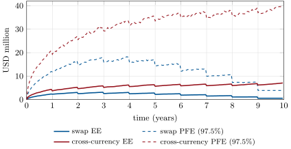
A bank receives fixed at the par rate of 3.80% on a USD 100 million ten-year swap (chapter 1’s SOFR curve, Hull–White with $\kappa = 3\%$ and a normal volatility of 90 basis points), and with the same counterparty receives USD fixed at 3.80% on USD 110 million and pays EUR fixed at the ESTR par rate of 2.59% on EUR 100 million for ten years, exchanging the notionals at the end (EURUSD at 1.10, volatility 8%). On 4 000 paths simulated every ten business days, the swap’s EE peaks at USD 3.13 million after three years and its PFE at USD 18.26 million after 3.9 years: rate risk grows with time and the remaining duration shrinks. The cross-currency swap’s EE rises to USD 7.09 million and its PFE to USD 39.93 million just before maturity, driven by the final exchange (Figure 17.1).

**Figure 17.1.** Exposure profiles of a ten-year interest rate swap (humped: uncertainty grows while the remaining cash flows run off) and a ten-year cross-currency swap (rising to maturity: the final exchange of notionals keeps the FX risk to the end). The small teeth are the annual payments. Data: the chapter’s tutorial.

17.2 Netting and collateral

Definition 17.5 (Netting set, close-out netting)

A netting set is the group of trades with one counterparty under one legally enforceable master agreement. Close-out netting lets the surviving party terminate every trade of the netting set on default and set the values off against each other into one net amount, so the exposure is $\max(\sum_iV_i,0)$ , not $\sum_i\max(V_i,0)$ .

As of September 2026 — Netting opinions

Whether close-out netting holds is a question of each counterparty’s insolvency law. ISDA has published legal opinions on the enforceability of netting under its master agreements covering over 90 jurisdictions, and on collateral covering over 60, generally updated every year.

Example 17.6 (The netting benefit)

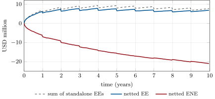
Netted, the two trades of Example 17.4 have an EE that peaks at USD 7.77 million after 3.9 years, where the two standalone EEs add to USD 9.24 million: a 16% saving (Figure 17.2). The netting set’s ENE reaches $-\text{USD}~21.0$ million: the bank pays the lower-rate currency and the final exchange is at a forward rate above spot, so the trade drifts in the counterparty’s favour.

**Figure 17.2.** Netting the swap and the cross-currency swap: the netted EE lies below the sum of the standalone EEs, and the netted ENE is larger in size than the EE because the netting set drifts in the counterparty’s favour. Data: the chapter’s tutorial.

The credit support annex of One Quant Book 2, chapter 10 makes the parties exchange variation margin as the netting set’s value moves. Three terms set how much.

Definition 17.7 (Collateral threshold, minimum transfer amount, independent amount)

The collateral threshold $\mathrm{Th}$ is the exposure a party accepts before calling for collateral: the collateral called is $V-\mathrm{Th}$ above it. The minimum transfer amount (MTA) is the smallest change in collateral that is called. The independent amount is collateral posted regardless of the value, a buffer against moves during the time it takes to close out.

17.3 Simulating exposure

Method 17.8 (Exposure by simulation)

(1) Choose a time grid, including the trades’ payment dates. (2) Simulate the risk factors jointly on the grid (here the Hull–White factor exactly, and EURUSD around its forward). (3) Revalue every trade on every path and date, in closed form where possible, by regression otherwise (the Longstaff–Schwartz method of One Quant Book 5). (4) Sum each netting set; apply the collateral agreement path by path. (5) Average and take quantiles across paths.

def simulate(m: Market, horizon: float, steps_per_year: int, paths: int, seed: int = 21) -> Scenarios:
    n = round(horizon * steps_per_year)
    times = np.arange(n + 1) / steps_per_year
    dt, k, s = 1.0 / steps_per_year, m.kappa, m.sigma
    rng = np.random.default_rng(seed)
    half = paths // 2
    x, fx = np.zeros((2 * half, n + 1)), np.zeros((2 * half, n + 1))
    fx[:, 0] = m.fx0
    e = math.exp(-k * dt)
    sd = s * math.sqrt((1 - e * e) / (2 * k))
    w = np.zeros(2 * half)
    for j in range(1, n + 1):
        t0, t1 = times[j - 1], times[j]
        drift = s * s / (2 * k) * ((1 - e) / k - math.exp(-k * t1) * (math.exp(-k * t0) - math.exp(-k * t1)) / k)
        z = rng.standard_normal((half, 2))
        z = np.concatenate([z, -z])
        x[:, j] = e * x[:, j - 1] + drift + sd * z[:, 0]
        w = w + math.sqrt(dt) * z[:, 1]
        fwd = m.fx0 * m.eur.df_t(t1) / m.usd.df_t(t1)
        fx[:, j] = fwd * np.exp(m.fx_vol * w - 0.5 * m.fx_vol ** 2 * t1)
    return Scenarios(times, x, fx, m)

Listing 17.1. Scenario generation: the Hull–White factor on the grid with its exact drift and variance, and EURUSD around its forward. code/firm/exposure/firm_exposure.py

The cost is paths times dates times trades times the cost of a valuation: millions of valuations for one netting set, billions for a bank. The revaluation step is where engines spend their time; the aggregation step (netting, collateral, profiles) runs over very large arrays and is the part the firm writes in C++20 and Rust.

17.4 The margin period of risk and the collateralised profile

Collateral does not remove the exposure: when a counterparty defaults, the last collateral it posted reflects the value at the last successful margin call, and the surviving party needs time to notice the failure, dispute, terminate and re-hedge.

Definition 17.9 (Margin period of risk)

The exposure under a collateral agreement at $t$ is $\max(V_t-C_{t-\delta},0)$ , where $\delta$ is the margin period of risk of One Quant Book 1: the collateral is the one agreed $\delta$ earlier. The exposure is the move of the netting set’s value over $\delta$ , plus the threshold and the minimum transfer amount.

def collateral(V: np.ndarray, threshold: float, mta: float) -> np.ndarray:
    """Two-way variation margin held (positive: received) agreed at each grid date."""
    C = np.zeros_like(V)
    for k in range(1, V.shape[1]):
        v = V[:, k]
        target = np.where(v > threshold, v - threshold, np.where(v < -threshold, v + threshold, 0.0))
        move = np.abs(target - C[:, k - 1]) >= mta
        C[:, k] = np.where(move, target, C[:, k - 1])
    return C


def exposure(V: np.ndarray, C: np.ndarray | None = None, lag: int = 0) -> np.ndarray:
    """Signed exposure V_k - C_{k - lag}: the collateral agreed one margin period of risk earlier."""
    if C is None:
        return V
    Cl = np.concatenate([np.zeros((V.shape[0], lag)), C[:, :V.shape[1] - lag]], axis=1) if lag else C
    return V - Cl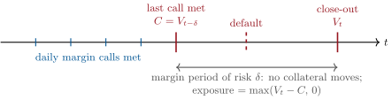

Listing 17.2. The collateral held under a two-way CSA, and the exposure that uses the collateral agreed one margin period of risk earlier. code/firm/exposure/firm_exposure.py

Figure 17.3. The margin period of risk: the last collateral received matches the value at the last successful call; between it and the close-out the counterparty posts nothing, and the value keeps moving. Schematic.

Example 17.10 (Collateralising the netting set)

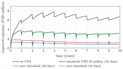
Under a two-way CSA with zero threshold and a minimum transfer amount of USD 500 000, the netting set’s EE falls to a nearly flat USD 1.30 million at its peak and its PFE to USD 6.45 million with a margin period of risk of ten business days; the EPE over the life falls from USD 6.44 million to 0.95 million, 15% of the uncollateralised figure. With twenty days the peak EE is USD 1.83 million, $\sqrt2$ times higher; with a threshold of USD 10 million it is USD 3.81 million (Figure 17.4).

Figure 17.4. Expected exposure of the netting set without collateral and under three CSAs. A zero-threshold CSA flattens the profile to the value moves over the margin period of risk; doubling that period multiplies them by about

\sqrt2

; a threshold adds exposure up to its size. The teeth at each anniversary are the annual payments, which the lagged collateral does not yet reflect. Data: the chapter’s tutorial.

As of September 2026 — Margin period of risk floors

The Basel Committee’s standardised approach for counterparty credit risk (March 2014) sets a minimum margin period of risk of ten business days for bilateral derivatives with daily margin, five for cleared client trades and twenty for netting sets of 5 000 or more transactions not with a central counterparty, doubled for netting sets with outstanding disputes; with margin every $N$ days it is $10+N-1$ days.

17.5 Wrong-way risk

Definition 17.11 (Wrong-way risk)

Wrong-way risk is a positive dependence between a counterparty’s probability of default and the bank’s exposure to it: the exposure is largest when default is likeliest. It is specific when the dependence is built into the trade (protection bought from a counterparty on itself or on its own country) and general when it comes through common market factors.

Example 17.12 (A counterparty that weakens with the euro)

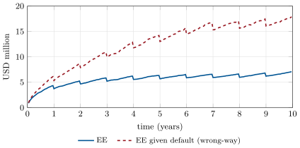
Let the counterparty of the cross-currency swap have a hazard rate of $2\%\times(X_t/F_X(0,t))^{-5}$ : a 10% fall of the euro below its forward raises its hazard by about 70%. The bank’s exposure is largest when the euro has fallen. Weighting the paths by the probability of default in each period, the expected exposure conditional on default is 2.52 times the unconditional EE at its peak, and 2.22 times on average over the life (Figure 17.5).

**Figure 17.5.** Expected exposure of the cross-currency swap, unconditionally and conditional on the counterparty defaulting at each date, when the counterparty’s hazard rises as the euro falls. The exposures that matter are those in the scenarios where the counterparty defaults. Data: the chapter’s tutorial.

As of September 2026 — Lehman’s derivatives

According to the Financial Crisis Inquiry Commission, Lehman first asserted around 930 000 derivative transactions at its bankruptcy; most had been terminated by 13 November 2008, 18 000 were still outstanding in January 2009, and by May 2010 banks had filed more than 50 billion dollars of claims for losses on derivatives with Lehman.

17.6 Tutorial: exposure of a netting set

Goal. Simulate the exposure of a swap, a cross-currency swap and their netting set, with and without variation margin. End state: the numbers of Examples 17.4, 17.6, 17.10 and 17.12 and their four charts.

Scenarios: simulate(MKT, 10, 26, 4000); check that EURUSD is a martingale around its forward.
Values: Swap.values(sc), XccySwap.values(sc); both are worth zero at the start.
Profiles: aggregate([swap]), the netting set, and the three CSAs.
Wrong way: wrong_way(); fig_rc_exposure.py writes the charts.

What to change next. Make the bank pay fixed on the swap and watch the netting benefit change; build the C++20 kernel (cpp/) and time it against the Python aggregation on 100 000 paths.

17.7 Build: the exposure engine

Purpose. The firm’s exposure engine: profiles of every netting set for credit limits (PFE), for the valuation adjustments of chapters 18 to 20 (EE, ENE), and for the risk engine of chapter 29.

Interface. Market, simulate(market, horizon, steps_per_year, paths, seed) returning Scenarios (usd_bond, eur_bond); trades Swap, XccySwap, FxForward with values(sc); collateral, exposure, profiles, epe, aggregate, conditional_ee. C++20 firm::exposure::aggregate (cpp/firm_exposure.hpp) and Rust firm_exposure::aggregate.

Rules. Risk-neutral scenarios; one grid step is the margin period of risk (ten business days); the final grid date, when all trades have matured, is excluded from profiles; PFE is the lower 97.5% quantile.

Acceptance tests. code/firm/exposure/tests/, cpp/ and rust/: the three implementations reproduce one fixture to $10^{-9}$ ; par trades are worth zero; FX and deflated bonds are martingales; netting and collateral reduce the peak EE, and a longer margin period of risk raises it.

Stretch. Cash flows during the margin period of risk; stochastic EUR rates and rate–FX correlation; regression revaluation of callable trades; the C++ kernel called from Python.

Sources and further reading

Basel Committee on Banking Supervision, The standardised approach for measuring counterparty credit risk exposures, March 2014.
Financial Crisis Inquiry Commission, The Financial Crisis Inquiry Report, 2011, notes to chapter 20.
J. Gregory, The xVA Challenge: Counterparty Risk, Funding, Collateral, Capital and Initial Margin, 4th edition, Wiley, 2020.

17.8 Exercises

Exercise 17.1 ★

Why is the expected exposure of an interest rate swap humped, and that of a cross-currency swap with final exchange increasing?

Solution

Solution of Exercise 17.1.

A swap’s value at $t$ is roughly the rate move to $t$ times the remaining annuity: the first grows like $\sqrt t$ , the second shrinks to zero, so the product peaks in between (about a third of the way for a swap). A cross-currency swap with a final exchange keeps the full notional’s FX risk until maturity, so its exposure keeps growing with $\sqrt t$ .

Exercise 17.2 ★

Two trades with one counterparty are worth $+10$ and $-7$ on a path. What is the exposure with and without close-out netting?

Solution

Solution of Exercise 17.2.

With netting, $\max(10-7,0) = 3$ ; without, the bank loses the $+10$ and must still pay the $7$ it owes: exposure 10.

Exercise 17.3 ★

A CSA has a threshold of USD 10 million and an MTA of USD 0.5 million; the netting set is worth USD 14.3 million and the bank holds USD 4.0 million. How much does it call?

Solution

Solution of Exercise 17.3.

The required collateral is $14.3-10 = 4.3$ million; the bank holds 4.0, so the change of 0.3 million is below the MTA of 0.5: no call.

Exercise 17.4 ★★

Why does doubling the margin period of risk multiply the collateralised EE by about $\sqrt2$ ?

Solution

Solution of Exercise 17.4.

With zero threshold the collateralised exposure is the value’s move over the margin period of risk, whose standard deviation scales with the square root of the period for a diffusion; EE is proportional to the standard deviation. The simulation gives 1.41.

Exercise 17.5 ★★

The netted ENE of Example 17.6 is larger in size than the EE. What does that mean for the counterparty, and for the bank’s DVA (chapter 18)?

Solution

Solution of Exercise 17.5.

The counterparty expects to be owed more by the bank than it owes: its exposure to the bank is larger than the bank’s to it. The bank’s DVA, the value of its own default to its creditors, is computed from the ENE and is correspondingly large.

Exercise 17.6 ★★

Give two examples of specific wrong-way risk and one of right-way risk.

Solution

Solution of Exercise 17.6.

Specific: buying protection on a country’s banks from one of those banks; a put on a company’s shares bought from the company. Right way: a commodity producer that sells its output forward to the bank owes the bank most when prices are high, which is when the producer is strongest.

Exercise 17.7 ★★★

Coding. Compute the peak EE of the netting set collateralised with a twenty-day margin period of risk and check the ratio to the ten-day figure.

Solution

Solution of Exercise 17.7.

USD 1.83 million against 1.30 million, a ratio of 1.41, close to $\sqrt2 = 1.414$ .

Exercise 17.8 ★★★

Find the flaw. “The counterparty posts daily variation margin with zero threshold, so our exposure to it is zero and it needs no credit limit.”

Solution

Solution of Exercise 17.8.

Margin lags: on default the bank holds the collateral of the last call met and bears the move over the margin period of risk (plus the MTA, disputes and settlement flows); the collateralised PFE of the chapter’s netting set is still USD 6.45 million. The counterparty needs a limit on that residual exposure, and on the risk that it stops posting.

17.9 Problem: The Uncollateralised Corporate

Problem 17.1

Weekend problem — signing a CSA

A corporate client pays fixed to the bank on a USD 50 million five-year swap (at the par rate) and buys EUR 20 million one year forward from the bank (at the forward rate). It has no CSA; the bank proposes one with zero threshold and a minimum transfer amount of USD 250 000, or one with a threshold of USD 5 million.

Part I — Without a CSA.

Give the swap’s par rate and the forward’s strike.
Give the netting set’s peak PFE and when it occurs.
Give its EPE over one year and over its life.
Which trade dominates the first year, and why?
Why does a corporate often refuse to sign a CSA?

Part II — With a CSA.

Give the peak PFE and the EPEs under the zero-threshold CSA.
Why does the collateralised PFE peak at one year exactly?
Give the peak PFE and the life EPE with the USD 5 million threshold.
Why does the USD 5 million threshold change almost nothing here?
What would the corporate need in order to post variation margin?

Part III — Limits and capital.

The bank’s limit for the client is a PFE of USD 4 million. Is the client within it?
How does the limit change the bank’s willingness to trade more?
How would the bank reduce the settlement-date PFE?
What happens to the exposure if the euro rises 10% in the first month?
Which party is exposed to whom on the FX forward if the euro falls?

Part IV — Judgement.

Why do banks still trade uncollateralised with corporates?
How would a margin period of risk of twenty days change the answers?
What does the bank give up by accepting a threshold?
State the named result: the peak PFE and the life EPE before and after the zero-threshold CSA.
In one sentence: what does a CSA turn a counterparty exposure into?

Solution

Solution of Problem 17.1.

1. 3.48%; 1.1166 dollars per euro. 2. USD 4.42 million, just before the forward settles at one year. 3. USD 626 224 over one year and 545 826 over five. 4. The forward: EUR 20 million at 8% volatility is larger risk than the swap in its first year, when little of the rate uncertainty has accumulated. 5. Posting cash daily needs liquidity and operations that most corporates do not have, and hedge accounting prefers stable cash flows. 6. Peak PFE USD 3.63 million; EPE USD 199 002 over one year and 97 606 over five. 7. The forward settles at one year: its value leaves the netting set as a payment while the collateral held still reflects it for one margin period of risk; if the bank had posted collateral against it, that collateral is exposed until returned. 8. Peak PFE USD 4.38 million; life EPE USD 544 793. 9. The netting set’s value rarely exceeds USD 5 million, so the threshold is seldom reached and almost no collateral would move. 10. Cash or securities to post, a treasury able to meet daily calls, and possibly a credit line for margin. 11. No: its peak PFE of USD 4.42 million exceeds the limit. 12. New trades that add exposure at the one-year peak need limit headroom; trades that reduce it (the client selling euros forward) are welcome. 13. A CSA, a shorter forward, settling the forward in two parts, or a break clause; payment-versus-payment settlement removes the delivery risk on the day. 14. The bank’s short euro forward loses about $20\text{ million}\times0.11 = \text{USD}~2.2$ million: its exposure to the client falls, the client’s exposure to the bank rises by as much. 15. If the euro falls the forward (bank sells euros at 1.1166) gains for the bank: the bank is exposed to the client. 16. Corporates generate the hedging business and have few alternatives; the bank charges for the exposure (chapters 18 to 20) and limits it. 17. Only the collateralised figures change, by about $\sqrt2$ on the residual exposure; the uncollateralised profile is unchanged. 18. Protection up to the threshold: the exposure below it stays uncollateralised and must be priced and limited. 19. Named result: the uncollateralised corporate: peak PFE USD 4.42 million and life EPE USD 545 826 without a CSA; USD 3.63 million and 97 606 with the zero-threshold CSA. 20. Into the risk of the value moving over a few days, plus the settlement flows.

17.10 Interview questions

Interview question 17.1 ★ risk, bank

Define EE, PFE and EPE. Which is used for what?

Solution

Solution of Interview question 17.1.

EE: the mean positive exposure at a date, used to price CVA. PFE: a high quantile of the exposure at a date, used for credit limits. EPE: the time average of EE, a single number used in regulatory exposure measures and in capital.

What the interviewer is looking for: the three definitions and their uses.

Interview question 17.2 ★★ developer, risk

Design an exposure simulation for a bank’s whole derivative book. Where does the time go?

Solution

Solution of Interview question 17.2.

Common scenarios for all risk factors on a grid; revaluation of every trade on every path and date (closed forms, grids, regression for callables), organised by trade type and vectorised; netting and collateral per netting set; profiles stored per netting set for the adjustments. The time goes into revaluation; the aggregation is memory-bound; both parallelise over paths.

What the interviewer is looking for: scenario, revaluation and aggregation, and where the cost is.

Interview question 17.3 ★★ risk

What is the margin period of risk and why is it not one day for a daily margined netting set?

Solution

Solution of Interview question 17.3.

The time between the last collateral received and the close-out and re-hedging of the defaulted netting set: noticing the missed call, disputes, grace periods, termination and replacement. Ten business days is the regulatory minimum for daily-margined bilateral trades, more for large or disputed netting sets.

What the interviewer is looking for: the steps in the period and the regulatory floors.

Interview question 17.4 ★★ trader, risk

Give an example of wrong-way risk and how you would measure it.

Solution

Solution of Interview question 17.4.

A bank buying protection on a sovereign from that sovereign’s banks; an FX forward in which a local company buys dollars and would default after a devaluation. Measure it by linking the counterparty’s hazard to the market factors in the simulation and computing exposure conditional on default, or by stress tests of joint scenarios.

What the interviewer is looking for: an example and a quantitative method.

Interview question 17.5 ★★★ researcher, developer

How do you compute the exposure of a Bermudan swaption inside a simulation?

Solution

Solution of Interview question 17.5.

Its value at each simulation date depends on the future exercise decision: use regression (Longstaff–Schwartz) on the simulated state to estimate the continuation value and the exercise indicator on each path, then its value on the path; after exercise, the trade becomes the underlying swap on that path.

What the interviewer is looking for: regression revaluation and path-dependent exercise.

Interview question 17.6 ★★★ risk, bank

What happened to Lehman’s derivative counterparties in the weeks after 15 September 2008?

Solution

Solution of Interview question 17.6.

They terminated their trades under the master agreements, netted, kept collateral, and replaced hedges in a stressed market all at once; most of the roughly 930 000 transactions were terminated within two months, some were still open in January 2009, and disputes over close-out amounts lasted years, with claims above 50 billion dollars.

What the interviewer is looking for: close-out, replacement cost and disputes.

Terms defined in this chapter

See all 2333 terms in the glossary