Rates, Credit, XVA and Risk · Rates, credit & risk
14Structural Credit Models
On 4 May 2005 General Motors’ share price rose 18% after Kirk Kerkorian offered to buy a large stake in the company: his company Tracinda then tendered for up to 28 million shares at 31 dollars each. The next day Standard & Poor’s cut the company’s debt two notches, to BB, below investment grade, and its bond and default-swap spreads widened. Trades that bet on the prices of the company’s debt and equity staying in line with each other lost on both legs, on consecutive days. The model behind many such trades is the subject of this chapter: a firm defaults when the value of its assets falls short of its debt, so that equity is an option on the firm and the prices of its shares and of its credit are two views of the same asset value. The reduced-form model of chapter 13 takes the hazard rate as given; the structural model explains it, and links it to the equity market, which is what makes it useful and what made May 2005 expensive.
14.1 Equity as a call on the firm
Definition 14.1 (Structural model)
A structural model of credit models the value of a firm’s assets and makes default an event defined by and the firm’s liabilities: assets below the debt at its maturity, or assets touching a barrier. Default is then predictable from the asset value, and the prices of equity and debt follow from it.
Definition 14.2 (Merton model)
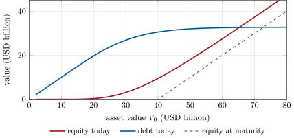
The Merton model takes assets following a geometric Brownian motion with volatility and one zero-coupon debt of face due at . At the shareholders receive and the creditors . Equity is a European call on the assets struck at the debt, priced by the Black–Scholes formula, and debt is the assets minus the equity:
Equivalently, debt is a riskless bond minus a put on the assets struck at : the creditors have sold the shareholders the right to hand over the firm instead of repaying. The credit spread of the debt is , and the risk-neutral probability of default is . Figure 14.1 shows the two claims as functions of the asset value.
The asset value and its volatility are not observed. Equity is: its market value and its volatility , implied from options or estimated from returns. By Itô’s formula on , , and with the pricing equation this gives two equations for the two unknowns.
def invert(E: float, sigma_E: float, D: float, T: float, r: float) -> tuple[float, float]:
    """Asset value and volatility matching equity value and equity volatility (Newton in two unknowns)."""
    V, s = E + D * math.exp(-r * T), sigma_E * E / (E + D * math.exp(-r * T))
    for _ in range(50):
        f1 = merton_equity(V, D, T, r, s) - E
        f2 = equity_vol(V, D, T, r, s) - sigma_E
        if abs(f1) < 1e-12 * E and abs(f2) < 1e-13:
            break
        hV, hs = 1e-6 * V, 1e-7
        a = (merton_equity(V + hV, D, T, r, s) - E - f1) / hV
        b = (merton_equity(V, D, T, r, s + hs) - E - f1) / hs
        c = (equity_vol(V + hV, D, T, r, s) - sigma_E - f2) / hV
        d = (equity_vol(V, D, T, r, s + hs) - sigma_E - f2) / hs
        det = a * d - b * c
        V -= (d * f1 - b * f2) / det
        s -= (a * f2 - c * f1) / det
return V, sExample 14.3 (A leveraged firm)
An illustrative firm has equity worth USD 10 billion with a volatility of 50%, and debt of face USD 40 billion treated as due in five years; . The inversion gives assets of USD 40.69 billion with a volatility of 15.6%: the equity is more than three times as volatile as the assets because it is levered. The debt is worth USD 30.69 billion, a yield spread of 130 basis points, and the risk-neutral probability that the assets end below the face is 32.7%.
14.2 Distance to default
Definition 14.4 (Distance to default)
The distance to default of a firm over a horizon is the number of standard deviations by which the expected log asset value exceeds the default point:
with the real-world asset drift. In the Merton model the real-world probability of default is ; in practice the distance is mapped to default frequencies through a history of defaults, because asset returns are not normal.
Example 14.5 (Two probabilities)
With an asset drift of 8%, the firm’s five-year distance to default is 1.02 and the real-world probability of default 15.4%, against the risk-neutral 32.7% of Example 14.3. The gap is the default risk premium of chapter 13 in structural form: under the risk-neutral measure the assets drift at instead of .
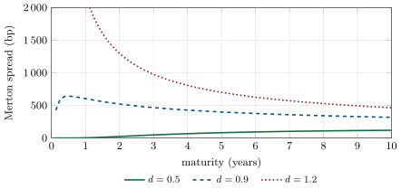
The Merton model’s term structure of spreads depends on the quasi-leverage (Figure 14.2). A firm with low leverage has spreads that start at zero and rise with maturity, since it takes time for the assets to fall to the debt; a firm near the default point has a humped curve; an insolvent one () has spreads falling with maturity, since only time can rescue it.
Remark 14.6 (Spreads that are too low)
Merton spreads are low for safe firms and short maturities: a diffusion cannot reach the default point in a few months, so short spreads are near zero while markets quote tens of basis points. Remedies add jumps to the assets, uncertainty about the default point, or a barrier that can be touched at any time, the next section.
14.3 First-passage models
Definition 14.7 (First-passage model, default barrier)
A first-passage model defaults the firm the first time its assets touch a default barrier below the current value, whenever that happens, instead of only at the debt’s maturity. A barrier stands for covenants that let creditors take over, or for the level at which the firm can no longer refinance. The CreditGrades model (2002), published by RiskMetrics with three dealers, puts the barrier at the average recovery on debt times the debt per share and makes that recovery lognormally uncertain, so that default can come as a surprise and short spreads are not zero.
Proposition 14.8 (Survival to a constant barrier)
With risk-neutral asset dynamics , a constant barrier , and , the probability of no default up to is
Proof. is a Brownian motion with drift and volatility ; the probability that it stays above up to follows from the reflection principle and a change of measure removing the drift (One Quant Book 4, chapter 2). ∎
def first_passage_survival(V: float, B: float, t: float, r: float, sigma: float, growth: float = 0.0) -> float:
    """P(min_{u<=t} V_u / (B e^{growth u}) > 1) for V with risk-neutral drift r (Black-Cox, reflection)."""
    if t <= 0.0:
        return 1.0
    nu = r - growth - 0.5 * sigma * sigma
    x = math.log(V / B)
    st = sigma * math.sqrt(t)
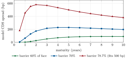
return ncdf((x + nu * t) / st) - math.exp(-2.0 * nu * x / (sigma * sigma)) * ncdf((-x + nu * t) / st)The survival function becomes a hazard curve on the premium dates, and chapter 13’s legs turn it into a model default-swap spread for each maturity, with a recovery set on the default swap’s convention (40%) rather than read from the asset value at the barrier.
Example 14.9 (The firm under a barrier)
With the barrier at 70% of the debt face, the firm’s model default-swap spreads are 64, 173, 216, 229 and 197 basis points at one, two, three, five and ten years (Figure 14.3); its five-year survival probability is 82.3%. A market quote of 500 basis points at five years needs a barrier at 78.7% of the face.
As of September 2026 — May 2005
The Bank for International Settlements’ review of June 2005 reported that on 4 May 2005 General Motors’ stock rose 18% after an offer from Kirk Kerkorian to buy a large stake, that on 5 May Standard & Poor’s cut GM by two notches to BB and Ford by one notch to BB+, and that relative-value trades between GM’s convertible bonds and a replicating portfolio lost on both legs as the bond and default-swap spreads rose.
14.4 Capital-structure signals and arbitrage
A structural model maps an equity price to a credit spread. Traders use the map in both directions: equity moves predict spread moves, and spreads far from the model’s value are candidate trades.
Definition 14.10 (Capital-structure arbitrage)
Capital-structure arbitrage trades one instrument of a firm’s capital structure against another (default swaps or bonds against equity or equity options) when their prices disagree with a structural model, hedging with the model’s sensitivity of one to the other: sell protection and short equity when the market spread is above the model’s, buy protection and buy equity when it is below.
Yu (2006) ran such a convergence strategy with CreditGrades on 135 759 daily default-swap spreads of 261 North American names: single trades could lose heavily because spreads and equity prices were weakly correlated, while an equally weighted portfolio of all trades earned Sharpe ratios similar to other fixed-income arbitrage strategies.
Method 14.11 (The equity hedge of a default swap)
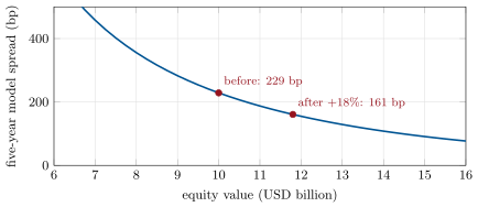
Hold the asset volatility fixed. Move the equity value by a small amount, find the asset value that reprices it, and recompute the model spread: this gives . Multiply by the position’s CS01 (per unit of spread) to get its value change per unit of equity value, and trade that much equity in the opposite direction.
Example 14.12 (The hedge ratio)
With the barrier at 70% of the face, the model spread falls by 0.47 basis points for each USD 0.01 billion rise in the equity value ( per USD billion). USD 10 million of sold five-year protection at the 500 coupon has a CS01 of per basis point at a quote of 500, so it gains USD 174 423 per USD 1 billion of equity value: the hedge is a short of USD 1.74 million of stock (Figure 14.4).
Remark 14.13 (What the model assumes about volatility)
Holding the asset volatility fixed makes the equity volatility fall as equity rises (leverage falls): after an 18% rally it is 47.1%. If instead the equity volatility stays at 50%, the inversion gives a higher asset volatility, 17.3%, and the model spread rises, to 251 basis points. The sign of the hedge depends on which volatility the desk believes is stable, and on equity options, if the firm has them.
14.5 Tutorial: from equity to spreads
Goal. Back out a firm’s assets from its equity, measure the distance to default, build model spreads in the Merton and first-passage models, and size an equity hedge. End state: the numbers of Examples 14.3, 14.9 and 14.12 and Figures 14.1, 14.2, 14.3 and 14.4.
- Invert:
invert(10, 0.5, 40, 5, 0.04); check equity and equity volatility reprice. - Merton:
firm()for the spread and both probabilities of default. - First passage:
fp_spreadfor each maturity andimplied_barrier()for the 500-basis-point quote. - Hedge:
hedge();fig_rc_structural.pywrites the charts.
What to change next. Let the barrier grow at the risk-free rate (growth) and compare the curves; recompute the hedge with the equity volatility held instead of the asset volatility.
14.6 Build: structural models
Purpose. The firm’s equity-to-credit map: model spreads for names with listed equity, the equity hedge of credit positions, and a check on default-swap marks.
Interface. merton_equity, merton_debt, merton_spread, merton_pd, distance_to_default, equity_vol; invert(E, sigma_E, D, T, r); asset_from_equity; first_passage_survival; hazard_curve_from_survival; model_cds_spread(q, r, maturity, recovery); FlatDisc.
Rules. Flat rate; one debt face; survival functions become hazard curves on the quarterly grid and are priced by chapter 13’s firm_cdscurve.
Acceptance tests. code/firm/structural/tests/: the inversion reprices equity and its volatility; debt plus equity is the assets and debt is below the riskless value; the first-passage formula reduces to the reflection principle without drift and to one with a vanishing barrier; a barrier defaults more than a terminal test; a flat survival gives chapter 13’s par spread.
Stretch. Barrier with uncertain level (a random recovery of the default point); jumps in the assets; a term structure of debt; the equity-option calibration of asset volatility.
Sources and further reading
- R. C. Merton, “On the pricing of corporate debt: the risk structure of interest rates”, Journal of Finance 29(2), 1974, 449–470.
- F. Black and J. C. Cox, “Valuing corporate securities: some effects of bond indenture provisions”, Journal of Finance 31(2), 1976, 351–367.
- F. Yu, “How profitable is capital structure arbitrage?”, Financial Analysts Journal 62(5), 2006, 47–62.
- C. C. Finger (ed.), CreditGrades Technical Document, RiskMetrics Group, May 2002.
- Bank for International Settlements, Quarterly Review, June 2005, box “Stress testing of credit markets: the downgrade of General Motors and Ford”.
14.7 Exercises
Exercise 14.1 ★
Assets 50, debt face 40 due in five years, asset volatility 20%, . Give the Merton equity and debt values, the yield spread and the risk-neutral probability of default.
Solution
Solution of Exercise 14.1.
Equity 18.89, debt , a yield spread of 103 basis points (), and a risk-neutral probability of default .
Exercise 14.2 ★
Why are Merton spreads near zero at short maturities for a healthy firm?
Solution
Solution of Exercise 14.2.
Assets follow a diffusion: to default within a few months they must fall from well above the debt to below it, which a continuous path with a volatility of 10–20% a year almost never does. The probability, and the spread, vanish faster than linearly as the maturity shrinks.
Exercise 14.3 ★
Give the one-year distance to default and the real-world probability of default of the chapter’s firm, with the same debt face and drift.
Solution
Solution of Exercise 14.3.
, a probability of default of 29.3%, higher than the five-year 15.4%: over one year the drift has had little time to lift the assets away from the face, and treating the whole face as due in one year overstates the risk. Practical distance-to-default measures use a default point of short-term debt plus part of the long-term debt for this reason.
Exercise 14.4 ★★
Without drift, a firm’s assets are 1.5 times the barrier with an asset volatility of 30%. Give the probability that it survives two years.
Solution
Solution of Exercise 14.4.
With the formula reduces to the reflection principle: .
Exercise 14.5 ★★
Size the equity hedge of USD 20 million of sold protection on the chapter’s firm.
Solution
Solution of Exercise 14.5.
The hedge is linear in the notional: twice USD 1.74 million, a short of USD 3.49 million of stock.
Exercise 14.6 ★★
Why is equity much more volatile than the assets, and why does the ratio change when the equity price moves?
Solution
Solution of Exercise 14.6.
: equity is a levered claim on the assets, so a given percentage move in the assets is a larger percentage move in the equity, by the ratio (3.2 for the chapter’s firm). When equity rises, leverage falls and the ratio falls: a fixed asset volatility means an equity volatility that falls as the price rises, the leverage effect.
Exercise 14.7 ★★★
Coding. Find the barrier that fits a five-year quote of 500 basis points, and give the model’s ten-year spread with that barrier.
Solution
Solution of Exercise 14.7.
implied_barrier() gives 78.7% of the face; the ten-year model spread with that barrier is 380 basis points, below the five-year 500 because the curve is humped.
Exercise 14.8 ★★★
Find the flaw. “The Merton model gives this firm 130 basis points and the market quotes 500. The default swap is 370 basis points too wide: sell protection.”
Solution
Solution of Exercise 14.8.
The Merton model is known to give spreads far below the market’s for most firms (no short-dated default, no jumps, no liquidity or risk premia beyond the diffusion’s), so a large gap is the norm, not a signal. A capital-structure trade compares the market with a model calibrated to the firm’s own history (the barrier), and trades changes in the gap, hedged; and a trade based on the level still needs the hedge and a view on why the gap should close.
14.8 Problem: The Capital-Structure Trade
Problem 14.1
Weekend problem — May 2005
A fund sees the chapter’s firm quoted at 500 basis points at five years while its first-passage model (barrier 70% of the face, fitted on the firm’s history) gives 229. It sells USD 10 million of five-year protection at the 500 coupon and shorts equity by the model’s hedge ratio. The next day the equity rises 18%; the day after, the firm is downgraded and the market spread widens by 200 basis points, to 700.
Part I — The trade.
- Give the model spread and the market spread, and the signal.
- Give the hedge ratio and the equity short.
- What does the fund earn while nothing happens?
- What view is the fund taking, stated without the model?
- Which risks does the hedge leave open?
Part II — The two days.
- Give the model spread after the 18% rally.
- Give the market spread the model predicted after the rally, applying the model’s change to the quote.
- Give the equity leg’s P&L.
- Give the default swap’s P&L had the market followed the model, and the hedged P&L.
- Give the default swap’s P&L at 700 and the total.
Part III — What the model missed.
- Give the hedge ratio after the rally.
- Recompute the model spread after the rally with the equity volatility held at 50%.
- Why can an equity rally and a spread widening happen together?
- At what market spread would the trade have broken even on the two days?
- Which instrument would have hedged the downgrade?
Part IV — Judgement.
- Why did many funds lose on similar trades in the same week?
- How would you size such trades?
- What would make you close the trade after the two days, and what would make you keep it?
- State the named result: the two legs’ P&L and the total on the two days.
- In one sentence: what does a structural model add to a credit desk?
Solution
Solution of Problem 14.1.
1. 229 and 500 basis points: the default swap is 271 basis points wide of the model, a signal to sell protection. 2. per USD billion; short USD 1.74 million of stock. 3. The 500-basis-point coupon on USD 10 million (USD 500 000 a year, before the cost of the equity short and its dividends, less funding income on the short’s proceeds). 4. That the firm’s credit is cheap relative to its equity: either spreads tighten or equity falls. 5. Default (jump-to-default of USD 6 million on the protection against a stock that falls to near zero), the model’s convexity, volatility, idiosyncratic moves in one leg (a takeover, a downgrade), and liquidity. 6. 161 basis points. 7. basis points. 8. . 9. on the default swap, a hedged P&L of (the convexity of Figure 14.4). 10. on the default swap; a total of . 11. per USD billion: the slope flattens as equity rises, so the hedge needs to be cut. 12. The asset volatility rises to 17.3% and the model spread goes to 251 basis points: in that version the model predicted a wider, not tighter, spread after the rally. 13. A takeover financed with debt, or a buyer of the shares whose interests differ from the creditors’, raises equity value and credit risk together: value moves from creditors to shareholders, which a model with fixed debt and a single asset value cannot produce. 14. 418 basis points: the default swap would have needed to tighten by 82 basis points to pay for the equity leg’s loss. 15. Nothing in the capital structure hedges a downgrade driven by the rating itself; index protection or protection on similar names hedges part of it, and a smaller position limits it. 16. Many held similar positions sized by similar models, so their unwinds moved prices against each other, as the BIS review described. 17. By the stress loss of both legs moving against the position together, not by the model’s hedged risk; with limits per name and on event risk. 18. Close if the event changed the firm (the debt will be downgraded further, the investor intends to change the capital structure); keep if the gap reflects forced selling and the firm is unchanged, with funding to wait. 19. Named result: the capital-structure trade in May 2005: the equity leg loses USD 313 961 and the default swap USD 689 903, a total of USD 1 003 863 on USD 10 million of protection over two days. 20. A link between the equity and credit prices of the same firm, for hedges, signals and names without liquid default swaps.
14.9 Interview questions
Interview question 14.1 ★ researcher, trader
Why is equity a call option on the firm? What is the debt?
Solution
Solution of Interview question 14.1.
Shareholders have limited liability: at the debt’s maturity they repay and keep the rest, or walk away and leave the assets to creditors. Their payoff is , a call on the assets struck at the debt. Debt is : a riskless bond minus a put on the assets.
What the interviewer is looking for: limited liability, the call, and debt as bond minus put.
Interview question 14.2 ★★ researcher, developer
How do you estimate a firm’s asset value and asset volatility?
Solution
Solution of Interview question 14.2.
Two equations in two unknowns: the equity value as a call on the assets, and the equity volatility as ; solve by Newton. Alternatives iterate on the asset return series implied by the daily equity values. The default point and horizon are choices, and the equity volatility can come from options.
What the interviewer is looking for: the two equations and the choices behind them.
Interview question 14.3 ★★ researcher
Why do structural models underprice short-dated credit, and how do you fix it?
Solution
Solution of Interview question 14.3.
Continuous asset paths cannot reach the default point quickly, so short-dated default probabilities are near zero. Fixes: jumps in the assets, an uncertain default barrier (the firm does not know exactly where it defaults), incomplete information about the assets, or a hybrid with a hazard rate.
What the interviewer is looking for: the diffusion reason and one or two fixes.
Interview question 14.4 ★★ risk, bank
What is a distance to default, and how is it turned into a probability of default in practice?
Solution
Solution of Interview question 14.4.
The number of asset standard deviations between the expected asset value and the default point at a horizon. Practitioners map it to default frequencies with an empirical table from historical defaults, because the normal tail understates default rates, and use a default point between short-term debt and total debt.
What the interviewer is looking for: the formula and the empirical mapping.
Interview question 14.5 ★★★ trader
Describe a capital-structure arbitrage trade and its hedge ratio. How can it lose on both legs?
Solution
Solution of Interview question 14.5.
Sell protection and short equity when the default swap is wide of a structural model calibrated to the firm (or the reverse), with the equity amount set by the model’s spread sensitivity to equity times the position’s CS01. It loses on both legs if the equity rallies (the short loses) while spreads widen (the protection loses), as when a leveraged buyout or a takeover bid moves value from creditors to shareholders, or a downgrade hits the debt alone.
What the interviewer is looking for: the hedge ratio and the both-legs scenario.
Interview question 14.6 ★★★ researcher, trader
Compare the reduced-form and structural approaches. When would you use each?
Solution
Solution of Interview question 14.6.
Reduced-form models fit the credit curve exactly and price credit derivatives consistently; they say nothing about why default happens. Structural models explain default from the balance sheet and link credit to equity, but fit market spreads poorly. Use reduced-form for pricing and risk of credit instruments; structural for names without default-swap quotes, equity-credit relative value, and credit scoring.
What the interviewer is looking for: fit versus explanation, and the use of each.