Strategies II: Volatility, Relative Value, Macro and the Bank Desks · Strategies

1Harvesting the Variance Risk Premium

At the end of 84% of months since 1990 the VIX index, the market’s price of the next month’s S&P 500 volatility, was higher than the volatility that followed: on average 19.5 against 15.4. Selling that price and delivering the realised volatility has been one of the most reliable trades in finance. Its losses come the other way, all at once. At the end of February 2020 the VIX stood at 40.1; the next month’s realised volatility was 94.5. On this chapter’s synthetic market a short-variance book earns a Sharpe ratio of 1.57 until its worst month, which then costs 7.7 of its monthly standard deviations: 22% of capital at a 10% volatility target, and more than the capital at 60%. This chapter is about the implementations of short volatility and about sizing them for the month that matters. The build is two components: firm.synthvol, the synthetic option market that Part I runs on, and firm.shortvol.

1.1 The premium and why it exists

The variance risk premium (Book 5, chapter 14) is the difference between the price of variance, the rate of a variance swap or the square of an index like the VIX, and the variance that is then realised. Carr and Wu measured it directly: they synthesised variance swap rates from option prices on five stock indexes and 35 stocks, and took the difference with realised variance as the premium. It is paid because variance is highest when investors are poorest: a long-variance position pays in crashes, and investors pay to hold it, as they pay for insurance.

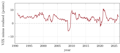
Definition 1.1 (Short-volatility strategy)

A short-volatility strategy earns the variance risk premium by selling options or variance and delivering realised volatility: short variance swaps, delta-hedged short options, covered calls, short puts, or short volatility futures. Its returns are small and frequent in calm markets and large and negative when volatility jumps.

The real record, from Cboe’s data (Figure 1.1): over 440 month-ends from January 1990 to August 2026 the VIX averaged 19.5% and the next month’s realised volatility of the S&P 500 15.4%; the VIX was higher 84% of the time, by 4.1 points on average; its square exceeded realised variance by 31% on average. The six months when it fell furthest short tell the other side: February 2020 (VIX 40.1, realised 94.5), September 2008 (39.4 and 82.3), August 2008 (20.6 and 54.3), March 2025 (22.3 and 47.7), July 2011 and June 2002.

The S&P 500 variance premium, 1990–2026: the twelve-month average, at each month-end, of the VIX minus the realised volatility of the S&P 500 over the following 21 trading days. Derived from Cboe’s VIX and S&P 500 index histories; the raw series are not redistributed. Data: s2_fetch_cboe. — **Figure 1.1.** The S&P 500 variance premium, 1990–2026: the twelve-month average, at each month-end, of the VIX minus the realised volatility of the S&P 500 over the following 21 trading days. Derived from Cboe’s VIX and S&P 500 index histories; the raw series are not redistributed. Data: `s2_fetch_cboe`.

1.2 Implementations: variance, options, overwriting

firm.synthvol (Listing 1.1) simulates twenty years of an index and thirty member stocks: a common factor with stochastic variance around 16% (mean reversion of four a year, a leverage correlation of $-0.7$ ), negative jumps once a year on average, and three planted crashes of 25%, 20% and 30% over ten days each. The truth sets the surface: the index’s at-the-money implied variance is the expected variance over the option’s life times 1.3, and the smile falls with strike. Realised volatility over the twenty years is 19.0%, crashes included, and the average one-month implied volatility 18.3%.

Definition 1.2 (Option overwriting)

Option overwriting sells options against a position already held, most often calls against a long equity position (covered calls), collecting premium in exchange for giving up gains beyond the strike; it is a short-volatility strategy with the market’s direction added.

firm.shortvol runs five monthly implementations on the index, each rolled every 21 trading days:

implementation, 239 months	Sharpe ratio	skewness	worst month (sd)	months up
short variance swap	0.69	$-3.53$	$-7.7$	79%
delta-hedged short straddle	1.24	$-2.32$	$-6.4$	77%
covered calls, 2% out of the money	0.40	$-4.24$	$-8.1$	69%
short puts, 5% out of the money	0.08	$-7.22$	$-10.2$	92%
short variance sized by $1/\text{strike}$	0.09	$-12.45$	$-14.2$	79%
the index itself	0.26	$-1.82$	$-6.8$	62%

Every implementation has negative skewness, and the shape matches the premium’s source: the short put wins in 92% of months and loses ten standard deviations in one. Sizing short variance by the inverse of its strike (more when volatility is cheap) makes it worse: the planted crashes start from calm markets, when the book is largest. The synthetic crashes are harsher than recent history: on Cboe’s indices from February 2007 to September 2026, PutWrite returned 7.2% a year at 13.8% volatility (a Sharpe ratio of 0.57 without a risk-free rate) and BuyWrite 6.0% at 14.3% (0.48), against 9.0% at 19.7% (0.53) for the S&P 500 price index, which omits dividends. PutWrite lost 27.6% from September to November 2008 and 19.8% in February and March 2020; BuyWrite 28.5% and 21.3%.

1.3 Delta-hedged option returns

Definition 1.3 (Delta-hedged option return)

A delta-hedged option return is the gain of an option position whose delta is hedged in the underlying at regular intervals, relative to its premium; under a model with no volatility risk premium its expectation is close to zero, so its sign and size measure the premium.

Bakshi and Kapadia used exactly this: in S&P 500 options, a delta-hedged long option underperformed zero, less so away from the money, more when volatility was high, even after accounting for jump fears. The seller’s side, a short at-the-money straddle hedged daily at the surface’s current volatility (Listing 1.2), earns 0.53% of the index a month on the synthetic market, about an eighth of the straddle’s premium of 4.2%, with a Sharpe ratio of 1.24, the best of the five, because the hedge removes the index’s own direction and leaves the gap between implied and realised volatility.

1.4 Blow-ups and how to size for them

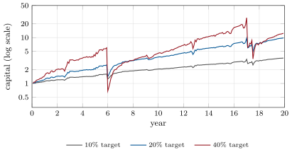
Short volatility is a sizing problem. Figure 1.2 scales the short-variance book to three volatility targets. Its Sharpe ratio before the worst month (the first crash, in year 5.9) is 1.57 at any size; the worst month costs 7.7 of its monthly standard deviations at any size:

target volatility	5%	10%	20%	40%	60%
Sharpe ratio before the worst month	1.57	1.57	1.57	1.57	1.57
worst month, share of capital	$-11.1\%$	$-22.2\%$	$-44.3\%$	$-88.6\%$	$-132.9\%$
capital survives	yes	yes	yes	yes	no

The record before the crash says nothing about the size of the crash: a manager who judged the risk from five years of monthly returns saw a Sharpe ratio above 1.5 and a worst month of a fraction of the one to come. The size that survives is set by the stress, not the volatility: a book that must not lose more than a quarter of its capital in a month can run the synthetic short-variance book at about 10% volatility, whatever its history.

The synthetic short-variance book scaled to three volatility targets, compounded monthly over twenty years; the planted crashes of years 6.0 and 17.5 show as single-month falls, the smaller one of year 12.7 barely. Data: s2_vrp.paths. — **Figure 1.2.** The synthetic short-variance book scaled to three volatility targets, compounded monthly over twenty years; the planted crashes of years 6.0 and 17.5 show as single-month falls, the smaller one of year 12.7 barely. Data: `s2_vrp.paths`.

1.5 Strategy files

Strategy file 1.1 — Short index variance

Who pays you, and why. Investors who pay for protection against variance, which is highest in bad times.

Instruments and venues. Variance swaps over the counter; a strip of listed options.

Signal. The variance premium: implied variance against a forecast of realised variance.

Sizing and execution. Sized by a stress (the worst plausible month), not by volatility; monthly rolls.

Costs. Option spreads on the replicating strip; dealer margins on swaps.

How it dies. Crashes; crowding, which raises the crash’s size.

Horizon, capacity, infrastructure. A month; large capacity in index variance; a surface and stress system.

Backtest honestly. Crash years in the sample; variance strikes as quoted; margin calls.

Sources. Carr and Wu (2009); Cboe VIX data; this chapter: 1.57 before the worst month, $-7.7$ standard deviations in it.

Strategy file 1.2 — Delta-hedged short straddle

Who pays you, and why. As for short variance, with the direction hedged away.

Instruments and venues. Listed at-the-money index options and futures for the hedge.

Signal. Implied against forecast volatility.

Sizing and execution. Sold monthly; delta hedged daily or on bands.

Costs. Option spreads and hedge trading.

How it dies. Gap moves the hedge cannot follow.

Horizon, capacity, infrastructure. A month; a hedging engine.

Backtest honestly. Hedges at executable prices; gaps and halts.

Sources. Bakshi and Kapadia (2003); this chapter: a Sharpe ratio of 1.24 on the synthetic index.

Strategy file 1.3 — Covered-call overwriting

Who pays you, and why. Buyers of upside calls; the variance premium on calls.

Instruments and venues. An equity holding and listed calls on it.

Signal. None beyond the premium; strike and tenor chosen by rule.

Sizing and execution. Calls written against the whole holding each month.

Costs. Option spreads; the upside given up.

How it dies. It does not die; it lags in strong rallies and falls with the market.

Horizon, capacity, infrastructure. A month; very large capacity.

Backtest honestly. Include dividends in the comparison index.

Sources. Cboe BuyWrite index: 6.0% a year at 14.3% volatility, 2007–2026.

Strategy file 1.4 — Put writing

Who pays you, and why. Buyers of crash protection, who pay most for out-of-the-money puts.

Instruments and venues. Listed index puts, collateralised with cash.

Signal. None beyond the premium.

Sizing and execution. Fully collateralised; one-month puts rolled at expiry.

Costs. Option spreads.

How it dies. Crashes: the short put wins most months and loses in a few.

Horizon, capacity, infrastructure. A month; very large capacity.

Backtest honestly. Collateral earning the bill rate; crash years in the sample.

Sources. Cboe PutWrite index: 7.2% a year at 13.8% volatility, 2007–2026; this chapter’s harsher synthetic crashes.

Strategy file 1.5 — Volatility-targeted short volatility

Who pays you, and why. As for short variance.

Instruments and venues. Variance swaps or straddles.

Signal. The premium, sized by current implied volatility.

Sizing and execution. Larger when implied volatility is low, smaller when high.

Costs. Extra turnover.

How it dies. Crashes that start from calm markets, when the book is largest.

Horizon, capacity, infrastructure. A month.

Backtest honestly. Crashes from low-volatility starts in the sample.

Sources. This chapter: sizing by the inverse of the strike cut the Sharpe ratio from 0.69 to 0.09.

1.6 Tutorial: picking up nickels

Goal. Build the synthetic option market, run five short-volatility implementations, and size the short-variance book through its planted crashes; compare with the real variance premium and option-writing indices. End state: the tables and the two figures.

The market: stochastic variance with leverage, jumps and crashes; members with specific returns.

def simulate_vol(cfg: VolConfig | None = None) -> dict:
    cfg = cfg or VolConfig()
    rng = np.random.default_rng(cfg.seed)
    T, N, dt = cfg.days, cfg.members, 1 / YEAR
    v = np.empty(T)
    r = np.empty(T)
    starts = {s: move for s, move in cfg.crashes}
    drift_left, vt = 0.0, cfg.theta
    for t in range(T):
        if t in starts:
            vt = max(vt, cfg.crash_var)
            drift_left = cfg.crash_days
            crash_move = starts[t]
        z1, z2 = rng.standard_normal(2)
        zv = cfg.rho * z1 + math.sqrt(1 - cfg.rho**2) * z2
        jump = rng.normal(cfg.jump_mean, cfg.jump_sd) if rng.random() < cfg.jump_rate * dt else 0.0
        r[t] = (cfg.mu - 0.5 * vt) * dt + math.sqrt(vt * dt) * z1 + jump
        if drift_left > 0:
            r[t] += crash_move / cfg.crash_days
            drift_left -= 1
        v[t] = vt
        vt = max(vt + cfg.kappa * (cfg.theta - vt) * dt + cfg.xi * math.sqrt(vt * dt) * zv, 1e-4)
    spec = cfg.spec_vol * np.exp(0.3 * rng.standard_normal(N))
    R = r[:, None] + spec[None, :] * math.sqrt(dt) * rng.standard_normal((T, N)) - 0.5 * spec**2 * dt
    return {"r": r, "v": v, "R": R, "spec": spec,
            "crashes": [(s, s + cfg.crash_days) for s, _ in cfg.crashes]}

Listing 1.1. Twenty years of the synthetic index and its members. code/firm/synthvol/firm_synthvol.py

Two implementations: the variance swap and the delta-hedged straddle.

def short_variance(r, v, cfg, tenor: int = 21):
    tau = tenor / YEAR
    out = []
    for s in periods(len(r), tenor):
        strike = float(atm_iv(v[s], cfg, tau)) ** 2
        realised = float((r[s + 1:s + 1 + tenor] ** 2).sum() / tau)
        out.append((strike - realised) * tau)
    return np.array(out)


def hedged_straddle(r, v, cfg, tenor: int = 21):
    out = []
    for s in periods(len(r), tenor):
        S, K = 1.0, 1.0
        vol0 = float(atm_iv(v[s], cfg, tenor / YEAR))
        premium = float(bs_price(S, K, tenor / YEAR, vol0, "C") + bs_price(S, K, tenor / YEAR, vol0, "P"))
        hedge_pnl = 0.0
        for d in range(tenor):
            tau = (tenor - d) / YEAR
            vol = float(atm_iv(v[s + d], cfg, tau))
            delta = float(bs_delta(S, K, tau, vol, "C") + bs_delta(S, K, tau, vol, "P"))
            S_new = S * np.exp(r[s + 1 + d])
            hedge_pnl += delta * (S_new - S)           # the short straddle's hedge is long its delta
            S = S_new
        out.append(premium - abs(S - K) + hedge_pnl)
    return np.array(out)

Listing 1.2. Short variance and a delta-hedged short straddle. code/firm/shortvol/firm_shortvol.py

Run s2_fetch_cboe.py once for the real statistics, then implementations(), leverage_table() and fig_vrp.py.

What to change next. Hedge the straddle on bands instead of daily; add a crash that starts from high volatility and see whether inverse-strike sizing helps; buy a far out-of-the-money put against the short variance and measure what it costs and saves.

1.7 Build: the synthetic option market and short volatility

Purpose. firm.synthvol: a deterministic index and member option market with stochastic variance, jumps, crashes and surfaces carrying a variance premium and a correlation premium, for Part I. firm.shortvol: short-volatility implementations and leverage.

Interface. VolConfig(…), simulate_vol(cfg), expected_var, atm_iv, smile_iv, bs_price, bs_delta; periods, short_variance, hedged_straddle, overwrite, put_write, lever.

Rules. Implied volatilities from the truth known at the time; options priced at the surface; P&L per unit of index at inception.

Acceptance tests. code/firm/synthvol/tests/ and code/firm/shortvol/tests/: Black–Scholes by hand, expected variance and the premium, a planted crash; variance and straddle P&L on a flat path, a wipe-out.

Stretch. Surfaces with term-structure premia; transaction costs on hedges; members’ options.

Sources and further reading

P. Carr and L. Wu, “Variance risk premiums”, Review of Financial Studies 22(3), 2009.
G. Bakshi and N. Kapadia, “Delta-hedged gains and the negative market volatility risk premium”, Review of Financial Studies 16(2), 2003.
Cboe Global Markets, daily histories of the VIX, S&P 500, PutWrite and BuyWrite indices.

1.8 Exercises

Exercise 1.1 ★

An at-the-money straddle is worth about $0.8\,\sigma\sqrt{\tau}$ of the index. What is it worth for a month (21 trading days) at 20% volatility?

Solution

Solution of Exercise 1.1.

$0.8 \times 0.20 \times \sqrt{21/252} = 0.8 \times 0.20 \times 0.289 = 4.6\%$ of the index.

Exercise 1.2 ★

Expected variance is $0.16^2$ and implied variance is 30% higher. What are the implied variance and volatility?

Solution

Solution of Exercise 1.2.

$0.16^2 \times 1.3 = 0.0333$ , an implied volatility of $\sqrt{0.0333} = 18.2\%$ against an expected 16%.

Exercise 1.3 ★

Why does the short put win more often than the short variance swap but have the lower Sharpe ratio?

Solution

Solution of Exercise 1.3.

The put is out of the money: it expires worthless in most months (92%) and pays the full premium, but in a crash its loss is many times the premium, a skewness of $-7.2$ ; the variance swap’s P&L is more even across months, so its mean is a larger share of its volatility.

Exercise 1.4 ★★

A book at 10% annual volatility loses 7.7 monthly standard deviations. What share of capital does it lose?

Solution

Solution of Exercise 1.4.

A monthly standard deviation is $10\%/\sqrt{12} = 2.9\%$ ; 7.7 of them are 22.2% of capital.

Exercise 1.5 ★★

Why does sizing short variance by the inverse of its strike make it worse on the synthetic market? When would it help?

Solution

Solution of Exercise 1.5.

The planted crashes start from calm markets, when implied variance and therefore the strike are low, so the book is largest exactly when the crash begins. Inverse-strike sizing would help if large losses followed high volatility, as when a volatile period continues rather than a calm one breaking.

Exercise 1.6 ★★

Why does the VIX exceed realised volatility most of the time, and why is its average excess not the premium’s full measure?

Solution

Solution of Exercise 1.6.

Investors pay for protection against variance, which rises when they are poorest. The average of VIX minus realised volatility includes the months when realised far exceeded the VIX; the premium is measured on variance, where those months weigh more, and over long samples that include crashes.

Exercise 1.7 ★★★

Coding. Run leverage_table((0.3, 0.5)). At which target volatility between them does the worst month take the whole capital?

Solution

Solution of Exercise 1.7.

At 30% the worst month costs 66.5% and the capital survives; at 50% it costs 110.8% and the capital is gone. The worst month is 7.68 monthly standard deviations, so the whole capital goes at a target of $1/(7.68/\sqrt{12}) = 45\%$ .

Exercise 1.8 ★★★

Find the flaw. “Our short-volatility fund has a Sharpe ratio of 2 over five years and its worst month was $-3\%$ ; at 15% volatility the risk is modest.”

Solution

Solution of Exercise 1.8.

Five calm years say nothing about the crash that the strategy is paid for bearing; the synthetic book’s history before its worst month also had a Sharpe ratio above 1.5. Size the fund by a stress (a month like February 2020 or October 2008 applied to today’s positions), not by its history.

1.9 Problem: Picking Up Nickels

Problem 1.1

Weekend problem — short volatility, sized

The chapter’s synthetic option market, Cboe’s data and the public record.

Part I — The premium.

Define a short-volatility strategy and option overwriting.
What did Carr and Wu measure, and how?
Give the VIX’s record against realised volatility, 1990–2026.
Name the months when realised volatility exceeded the VIX by most.

Part II — Implementations.

Describe the synthetic market and how its surface is set.
Give the five implementations’ Sharpe ratios and skewness.
Why is every skewness negative?
What did the PutWrite and BuyWrite indices earn, and how did they fare in 2008 and 2020?

Part III — Hedged options.

Define a delta-hedged option return.
What did Bakshi and Kapadia find?
What does the synthetic straddle earn, and why is its Sharpe ratio the highest?
What would a hedge on bands change?

Part IV — The verdict.

State the named result: the short-variance book’s Sharpe ratio before its worst month and its loss in that month, by leverage.
Why does the record before the crash not measure the crash?
How should a short-volatility book be sized?
Why did inverse-strike sizing fail here?
How would you backtest a short-volatility strategy honestly?
Which strategy file wins most often, and which has the best Sharpe ratio?
How does this chapter relate to Book 8, chapter 26’s volatility targeting?
In one sentence: what does a short-volatility trader sell?

Solution

Solution of Problem 1.1.

Selling options or variance to earn the premium; selling options against a position held, most often calls.
The variance risk premium as realised variance minus a variance swap rate synthesised from options, on five indexes and 35 stocks.
VIX 19.5 against realised 15.4 on average, higher in 84% of months, by 4.1 points; variance 31% higher.
February 2020, September and August 2008, March 2025, July 2011, June 2002.
Stochastic variance with leverage, jumps and three crashes; implied variance 1.3 times expected variance, a falling smile.
0.69, 1.24, 0.40, 0.08 and 0.09; skewness from $-2.3$ to $-12.5$ .
The premium is paid for bearing crashes: small gains most months, large losses rarely.
PutWrite 7.2% a year (Sharpe 0.57), BuyWrite 6.0% (0.48); $-27.6\%$ and $-28.5\%$ in autumn 2008, $-19.8\%$ and $-21.3\%$ in early 2020.
The gain of a delta-hedged option relative to its premium, which measures the volatility premium.
Delta-hedged long index options underperform zero, less away from the money, more when volatility is high.
0.53% of the index a month, about an eighth of the premium; the hedge removes the index’s direction.
Fewer hedge trades and more path dependence: lower costs, noisier P&L.
Named result. The short-variance book’s Sharpe ratio before its worst month is 1.57 at any size; the worst month costs 11.1%, 22.2%, 44.3% and 88.6% of capital at 5%, 10%, 20% and 40% volatility, and more than the capital at 60%.
The crash is a single rare event; five calm years contain no information about its size.
By a stress on today’s positions, so that the worst plausible month is survivable.
It sized up in calm markets, where the crashes began.
Crash years in the sample, executable option prices, margin calls, and a direct comparison with the underlying.
Put writing wins most often (92% of months); the hedged straddle has the best Sharpe ratio.
Volatility targeting cuts risk after volatility rises; here the losses come as volatility rises, faster than a target can react.
Insurance against variance.

1.10 Interview questions

Interview question 1.1 ★ researcher

What is the variance risk premium, and why does it exist?

Solution

Solution of Interview question 1.1.

The difference between the price of variance (implied) and the variance then realised; it is positive on average because variance is high in bad times and investors pay to hedge it.

Interview question 1.2 ★★ trader

You are short a delta-hedged straddle and the index gaps down 5% overnight. What happened to your P&L, and what do you do?

Solution

Solution of Interview question 1.2.

The straddle’s gamma loss is about $\tfrac12\Gamma(\Delta S)^2$ , large for a 5% gap, and implied volatility rises too (a vega loss); re-hedge the new delta at the open, check the stress limit, and cut if the book is beyond it rather than wait for a rebound.

Interview question 1.3 ★★ risk

How would you set limits on a short-volatility book?

Solution

Solution of Interview question 1.3.

With stress limits on the loss in historical and hypothetical crashes applied to current positions, vega and gamma limits by tenor, a cap on the premium collected relative to capital, and liquidity limits on how fast the book can be cut.

Interview question 1.4 ★★ researcher

Compare selling variance swaps, straddles and out-of-the-money puts as ways to earn the premium.

Solution

Solution of Interview question 1.4.

Variance swaps take the premium across all strikes and have a clean, convex payoff with crash exposure in the tail; straddles take it at the money with delta hedging and path dependence; out-of-the-money puts take the richest part of the skew with the most concentrated crash risk.

Interview question 1.5 ★★ developer

What does a daily delta-hedging engine for an option book need?

Solution

Solution of Interview question 1.5.

Positions and prices, a surface for each underlying, Greeks by option, aggregation by underlying, a hedging rule (time or bands), order generation in the hedge instrument, and reconciliation of hedge fills against the model.

Interview question 1.6 ★★★ researcher

A delta-hedged option with gamma $\Gamma$ on an underlying at $S$ is hedged continuously. Show that its P&L over a short interval is about $\tfrac12\Gamma S^2(\sigma_r^2 - \sigma_i^2)\,dt$ , with $\sigma_r$ realised and $\sigma_i$ implied volatility, and explain what this implies for its sign.

Solution

Solution of Interview question 1.6.

The hedged position’s change is $\tfrac12\Gamma(dS)^2 + \Theta\,dt$ ; with $\Theta = -\tfrac12\Gamma S^2\sigma_i^2$ (Black–Scholes at implied volatility) and $(dS)^2 = S^2\sigma_r^2\,dt$ , the P&L is $\tfrac12\Gamma S^2(\sigma_r^2 - \sigma_i^2)\,dt$ : a long option earns when realised exceeds implied, a short one when implied exceeds realised, weighted by gamma.

Terms defined in this chapter

See all 2333 terms in the glossary