Strategies II: Volatility, Relative Value, Macro and the Bank Desks · Strategies
20Mortgage and Structured-Credit Strategies
A homeowner can repay a mortgage whenever rates fall, so a mortgage bond is short an option that borrowers may not exercise well. A trader who models the borrowers better than the market is paid for it, and one who models them worse pays. Gabaix, Krishnamurthy and Vigneron found that prepayment risk, which washes out in the aggregate, is nonetheless priced, as if the marginal investor were a specialist rather than a diversified investor. On this chapter’s synthetic pool the market’s prepayment model assumes mild burnout. An interest-only strip bought on the view that burnout is strong and hedged with Treasuries gains 35.8% of its price if the view is right. If borrowers never burn out, it loses 25.5%. The build is firm.mbsrv.
20.1 Prepayment views
Definition 20.1 (Prepayment trade)
A prepayment trade is a position in mortgage securities whose value depends on how fast borrowers repay (pass-throughs of one coupon or pool type against another, interest-only or principal-only strips), taken because the trader’s prepayment model differs from the one in the market’s prices, with the interest-rate risk hedged away.
The market’s model in firm.mbsrv is Book 6’s (chapter 12): housing turnover on the PSA ramp, a refinancing S-curve in the incentive (the borrowers’ rate less the current mortgage rate) with a maximum CPR of 45%, and burnout that decays refinancing by a factor , where is the cumulative positive incentive in percentage-point years. The pool pays its borrowers’ 6.5% to investors less 50 basis points, has 29 years left, and is priced on Hull-White rate paths around a flat 4% curve at an option-adjusted spread of 50 basis points. New mortgages cost about 5.8%, so the borrowers already have an incentive to refinance.
A trader believes these borrowers have passed up refinancing before and will keep passing it up: burnout of 1.0 instead of 0.25. If so, the pool prepays more slowly than the market expects, and the interest-only strip, which is paid only while principal is outstanding, is worth more.
20.2 Interest-only and principal-only trades
The IO is worth 26.05 per 100 of pool face under the market’s model. Its value rises with rates, since higher rates slow refinancing, so hedging it means buying Treasuries: 0.51 ten-year Treasuries of face 100 per IO, the ratio that cancels the IO’s rate risk as the market’s model measures it (Listing 20.1). The trade’s gain is the IO’s value under the model that turns out to be true, at the same option-adjusted spread, less the price paid, plus the hedge.
| borrowers behave as | hedged gain, rates unchanged | rates 100 bp lower |
|---|---|---|
| the market’s model (burnout 0.25) | 0.0% | 10.1% |
| the view (burnout 1.0) | 35.8% | 63.6% |
| slower refinancing (maximum CPR 33%) | 16.4% | 31.1% |
| never burning out (burnout 0) |
The trade is a bet on borrowers, not on rates, but rates decide how much the bet matters (Figure 20.1). When rates fall the incentive grows, and whether borrowers act on it is the whole question. The view gains more and the wrong burnout assumption loses more. When rates rise the incentive disappears, and every model predicts the same slow turnover. Even under the market’s own model the hedged IO gains in large moves either way, because the hedge is sized for small ones.
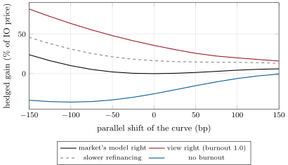
s2_mbsrv.io_scenarios.The principal-only strip is the mirror: it gains when prepayments are fast, so the trader who believes borrowers will refinance more than the market expects buys the PO. The pair of strips lets a trader take either side of a prepayment view with the same pool.
The coupon stack
The same view reprices every coupon. Pools whose borrowers pay more (higher coupons) have more incentive to refinance, so a model with stronger burnout values them more. At the market’s prices, the view’s option-adjusted spread rises from 59 basis points on the 4.0% coupon to 148 on the 7.5% (Figure 20.2). Under a model without burnout, the same prices give OASs falling from 42 to basis points. An OAS relative-value trade buys the coupon with the highest OAS under the trader’s model and sells the lowest, hedged in duration. The trade earns the OAS difference only if the model is right.
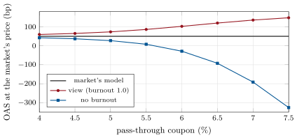
s2_mbsrv.stack.Real OASs are not flat across coupons either. Boyarchenko, Fuster and Lucca found that MBS spreads show a pronounced smile across coupons, and attributed the smile to prepayment risk that is not interest-rate risk, identified from the prices of stripped MBS. The time-series variation of spreads, by contrast, was mostly explained by risks other than prepayment. A smile across coupons is what a market pricing borrowers’ behaviour as a risk, not a known function, would produce; it is also what a trader with the wrong model would see as mispricing.
20.3 Tranche relative value
Definition 20.2 (Tranche relative value)
Tranche relative value is trading one tranche of a pooled credit structure against another, or against the index or the underlying names, because the trader’s model of default correlation or of the pool’s losses differs from the one in the tranches’ prices.
The large-pool Gaussian copula of Book 2 (chapter 24) prices tranches from the pool’s default probability and one correlation. With a five-year default probability of 6% and 40% recovery, the pool’s expected loss is 3.6% whatever the correlation. The tranches split it very differently as correlation changes:
| expected loss, % of tranche | correlation 0.15 | 0.30 | 0.45 |
|---|---|---|---|
| equity 0–3% | 74.45 | 59.86 | 48.11 |
| mezzanine 3–7% | 25.32 | 24.34 | 22.11 |
| mezzanine 7–10% | 7.52 | 11.69 | 13.00 |
| senior 10–15% | 2.10 | 5.70 | 7.92 |
| super senior 15–30% | 0.15 | 1.23 | 2.77 |
The senior tranche’s expected loss is eighteen times larger at a correlation of 0.45 than at 0.15; the pool’s is unchanged. Coval, Jurek and Stafford named this fragility as one of two features that explain the rise and fall of structured finance: ratings that change drastically with modest errors in the underlying risks, and exposure to systematic risk. In a companion paper they found that many structured products paid off like economic catastrophe bonds, defaulting only in severe downturns, while offering far less compensation than alternatives with comparable payoffs.
A trader who believes the correlation is 0.15 while the market prices at 0.30 sells protection on the 7–10% tranche and is paid the market’s expected loss of 11.7% of the tranche over five years (Listing 20.2). On 4 000 simulated pools of 125 names:
| true correlation | mean gain (% of tranche) | chance of a loss | tranche wiped out |
|---|---|---|---|
| 0.15 (the view) | 3.1 | 11.3% | 5.4% |
| 0.30 (the market) | 14.5% | 9.4% | |
| 0.45 | 15.0% | 10.9% |
Even when the view is right, the seller loses the whole tranche in 5.4% of pools, about one in twenty. The small loss at the market’s own correlation comes from the finite pool of 125 names, which the large-pool formula ignores. A tranche view is a view on the tail, and a few years of history cannot confirm it.
20.4 Strategy files
Strategy file 20.1 — IO long on a slow-prepayment view
Who pays you, and why. Holders of prepayment risk who price borrowers with a generic model; specialists are the marginal investors.
Instruments and venues. Interest-only strips of agency pools; Treasuries or swaps to hedge.
Signal. A prepayment model by pool characteristics (loan size, seasoning, past incentive) against the market’s speeds.
Sizing and execution. Hedge the rate risk the market’s model measures; size for the model being wrong.
Costs. Wide bid-ask on strips; hedge rebalancing.
How it dies. A refinancing wave the model underestimates; a policy change that makes refinancing easier.
Horizon, capacity, infrastructure. Years; loan-level data and a prepayment model.
Backtest honestly. Out-of-sample speeds by cohort; the model re-estimated only on data available at the time.
Sources. Gabaix, Krishnamurthy and Vigneron (2007); this chapter: if right, with no burnout.
Strategy file 20.2 — OAS relative value across coupons
Who pays you, and why. Investors who hold coupons for reasons other than their OAS: banks, the central bank, index trackers.
Instruments and venues. TBAs and specified pools across the coupon stack; dollar rolls.
Signal. Each coupon’s OAS under the trader’s model.
Sizing and execution. Long high-OAS, short low-OAS coupons, duration-hedged.
Costs. Roll financing; specified-pool payups.
How it dies. The model’s error, which is the OAS; supply from new issuance at one coupon.
Horizon, capacity, infrastructure. Months.
Backtest honestly. OAS from the model as it was, not refitted.
Sources. Boyarchenko, Fuster and Lucca (2019); this chapter: an 88 basis point OAS difference under the view.
Strategy file 20.3 — Mezzanine tranche relative value
Who pays you, and why. Buyers or sellers of protection at one level of a structure for reasons other than its price: rating constraints, hedging, regulatory capital.
Instruments and venues. Index tranches; the index; CLO or CMBS tranches in cash form.
Signal. Correlation or pool-loss views against the tranches’ implied correlations.
Sizing and execution. Delta-hedged with the index; size for the wipe-out.
Costs. Wide bid-ask; model risk in the hedge ratio.
How it dies. A systematic default wave; correlation that jumps.
Horizon, capacity, infrastructure. Years; a copula and a pool-loss model.
Backtest honestly. Stress the tail; history is too short to confirm a correlation view.
Sources. Coval, Jurek and Stafford (2009); this chapter: mean, wiped out in 5.4% of pools.
20.5 Tutorial: better than the market’s model
Goal. Price a pool, its strips and its coupons with one prepayment model, revalue them with another, and sell protection on a tranche at the wrong correlation. End state: the three tables and two figures.
The IO trade and the coupon stack.
def io_trade(cfg: MbsConfig, market: PrepayModel, truth: PrepayModel, side: float = 1.0, shifts=(0.0,),
             dy: float = 0.0025) -> dict:
    """Buy (side +1) or sell (-1) the IO at the market model's value, and hedge the rate risk the market model measures
    with the ten-year Treasury. For each parallel shift of the curve: the IO's value under the true model less the
    price paid, plus the hedge's change; in % of the price."""
    price = strip_paths(cfg, market)["io"].mean()
    dv_io = strip_paths(cfg, market, shift=-dy)["io"].mean() - strip_paths(cfg, market, shift=dy)["io"].mean()
    t0 = _treasury(cfg).mean()
    hedge = -dv_io / (_treasury(cfg, -dy).mean() - _treasury(cfg, dy).mean())   # Treasuries (face 100) per IO
    gains = []
    for s in shifts:
        io = strip_paths(cfg, truth, shift=s)["io"].mean()
        gains.append(side * (io - price + hedge * (_treasury(cfg, s).mean() - t0)) / price * 100)
    return {"price": float(price), "hedge": float(side * hedge), "gain": np.array(gains)}


def coupon_stack(cfg: MbsConfig, market: PrepayModel, view: PrepayModel, wacs) -> list[dict]:
    """For each borrowers' rate: the market model's price at the market OAS, the OAS the view model needs to return
    that price, and the market model's effective duration."""
    out = []
    for w in wacs:
        m = strip_paths(cfg, market, w)
        price = float(m["pt"].mean())
        v = strip_paths(cfg, view, w)
        oas_view = solve_oas(price, v["flows"], v["rs"])
        up = strip_paths(cfg, market, w, shift=0.0025)["pt"].mean()
        dn = strip_paths(cfg, market, w, shift=-0.0025)["pt"].mean()
        dur = float((dn - up) / (2 * price * 0.0025))
        out.append({"wac": w, "price": price, "oas_view": oas_view, "duration": dur})
    return out
Listing 20.1. Buying the IO on a view, hedged; each coupon’s OAS under the view. code/firm/mbsrv/firm_mbsrv.py The tranche.
def tranche_rv(p: float = 0.06, rho_market: float = 0.30, rho_true: float = 0.15, attach: float = 0.03,
               detach: float = 0.07, recovery: float = 0.40, names: int = 125, trials: int = 4000,
               seed: int = 163) -> dict:
    """Expected loss of [attach, detach] at both correlations (share of the tranche); selling protection at the
    market's expected loss earns it and pays the loss realised on pools simulated at the true correlation."""
    el_m = expected_tranche_loss(attach, detach, p, rho_market, recovery)
    el_t = expected_tranche_loss(attach, detach, p, rho_true, recovery)
    losses = np.array([tranche_loss(x, attach, detach) for x in simulate_pool(names, p, rho_true, recovery, trials,
                                                                               seed)])
    pnl = el_m - losses
    return {"el_market": el_m, "el_true": el_t, "pnl_mean": float(pnl.mean()), "pnl_q05": float(np.quantile(pnl, 0.05)),
            "p_loss": float((pnl < 0).mean()), "wipeout": float((losses >= 1.0).mean())}
Listing 20.2. Selling protection at the market’s correlation, paid on pools at the true one. code/firm/mbsrv/firm_mbsrv.py The four truths.
CFG = MbsConfig()
MARKET = PrepayModel()
TRUTHS = {"market": MARKET, "view": PrepayModel(burnout=1.0), "slow": PrepayModel(refi_top=0.33),
          "no_burnout": PrepayModel(burnout=0.0)}
SHIFTS = tuple(range(-150, 151, 25))
WACS = (0.045, 0.05, 0.055, 0.06, 0.065, 0.07, 0.075, 0.08)
TRANCHES = ((0.0, 0.03), (0.03, 0.07), (0.07, 0.10), (0.10, 0.15), (0.15, 0.30))


@functools.lru_cache(maxsize=1)
def io_scenarios() -> dict:
    """Hedged gain (% of the IO's price) of buying the IO at the market's value, by parallel shift (bp), per truth."""
    out = {n: io_trade(CFG, MARKET, m, 1.0, [s * 1e-4 for s in SHIFTS]) for n, m in TRUTHS.items()}
    return {"price": out["market"]["price"], "hedge": out["market"]["hedge"],
            "gain": {n: [float(g) for g in r["gain"]] for n, r in out.items()}}
Listing 20.3. The market’s model, the view and two alternatives. code/strategies-2/20-mortgage-and-structured-credit-strategies/python/s2_mbsrv.py - Run
io_summary(),stack(),tranches(),mezz()andfig_mbsrv.py.
What to change next. Draw the true burnout at random and measure the trade’s distribution; hedge the IO with the market’s model and then with the view’s; delta-hedge the tranche with the index.
20.6 Build: mortgage and structured-credit relative value
Purpose. Prepayment-view trades on Book 6’s OAS model and Book 2’s tranche model.
Interface. MbsConfig(…), FlatCurve(rate), strip_paths(cfg, model, wac, oas, shift), io_trade(cfg, market, truth, side, shifts), coupon_stack(cfg, market, view, wacs), tranche_rv(p, rho_market, rho_true, …).
Rules. Prices from the market’s model at one OAS; values under the true model at the same OAS; hedges sized with the market’s model.
Acceptance tests. code/firm/mbsrv/tests/: IO plus PO is the pass-through; no gain when the truth is the market’s model; the same model returns the market’s OAS; equal correlations give equal expected losses.
Stretch. Loan-level pools; dollar rolls; CLO waterfalls.
Sources and further reading
- X. Gabaix, A. Krishnamurthy and O. Vigneron, “Limits of arbitrage: theory and evidence from the mortgage-backed securities market”, Journal of Finance 62(2), 2007.
- N. Boyarchenko, A. Fuster and D. O. Lucca, “Understanding mortgage spreads”, Review of Financial Studies 32(10), 2019.
- J. Coval, J. Jurek and E. Stafford, “The economics of structured finance”, Journal of Economic Perspectives 23(1), 2009.
- J. Coval, J. Jurek and E. Stafford, “Economic catastrophe bonds”, American Economic Review 99(3), 2009.
20.7 Exercises
Exercise 20.1 ★
An IO bought at 26.05 per 100 of face gains 35.8% of its price. What is the gain per 100 of face?
Solution
Solution of Exercise 20.1.
per 100 of face.
Exercise 20.2 ★
Under the view, the 7.5% coupon’s OAS is 148 basis points and the 4.0% coupon’s 59; without burnout they are and 42. What OAS difference does a long 7.5%, short 4.0% trade earn in each case?
Solution
Solution of Exercise 20.2.
Under the view basis points (from the unrounded values); without burnout basis points. The same prices give a large gain or a large loss depending on the model.
Exercise 20.3 ★
The 7–10% tranche of an index with notional 1 billion has an expected loss of 11.69% of the tranche. What is the expected loss in money?
Solution
Solution of Exercise 20.3.
The tranche is 3% of the index, 30 million; million.
Exercise 20.4 ★★
Why does an IO lose value when rates fall, and why is hedging it a purchase of Treasuries?
Solution
Solution of Exercise 20.4.
The IO is paid interest only on the principal still outstanding. When rates fall, borrowers refinance, principal disappears and the interest with it, so the IO loses. Its value therefore rises with rates, like a short bond position, and hedging a short-bond exposure means buying bonds.
Exercise 20.5 ★★
Why would prepayment risk, a wash in the aggregate, carry a price?
Solution
Solution of Exercise 20.5.
Gabaix, Krishnamurthy and Vigneron found that it is priced as if the marginal investor were a specialised MBS arbitrageur, for whom prepayment risk is not diversified away: what is a wash for the economy is concentrated in the books of the few who hold and hedge mortgages.
Exercise 20.6 ★★
Why is a senior tranche’s rating fragile when the pool’s expected loss is well estimated?
Solution
Solution of Exercise 20.6.
A senior tranche loses only when many names default together, so its expected loss depends on correlation, which is hard to estimate, not on the pool’s expected loss alone. In the chapter’s table the super-senior tranche’s expected loss is eighteen times larger at a correlation of 0.45 than at 0.15 for the same pool; Coval, Jurek and Stafford named this fragility of ratings to modest errors as one cause of the collapse of structured finance.
Exercise 20.7 ★★★
Coding. Rerun the IO trade with MbsConfig(sigma=0.012). How do the price, the view’s gain and the no-burnout loss change?
Solution
Solution of Exercise 20.7.
The IO’s price rises from 26.05 to 26.85, the view’s gain falls from 35.8% to 33.5% and the no-burnout loss grows from 25.5% to 26.5%. More volatility sends more paths into deep refinancing, where the wrong burnout assumption costs most, so the view’s edge shrinks against its downside; a prepayment view is also a view on rate volatility.
Exercise 20.8 ★★★
Find the flaw. “The 7.5% coupon’s OAS is 148 basis points against 59 for the 4.0%: it is 88 basis points cheap, and we lock that in.”
Solution
Solution of Exercise 20.8.
The OAS is an output of the model: at the same prices, a model without burnout gives the 7.5% coupon an OAS of basis points and the 4.0% one 42, a difference of . Nothing is locked in; the 88 basis points are earned only if borrowers behave as the view’s model says, and the hedge ratios depend on the model too.
20.8 Problem: Better Than the Market’s Model
Problem 20.1
Weekend problem — mortgage and structured credit
The chapter’s synthetic pool and tranches and the public record.
Part I — The pool.
- Define a prepayment trade.
- Describe the market’s prepayment model and the pool.
- What is burnout, and what does the view assume?
- What did Gabaix, Krishnamurthy and Vigneron find?
Part II — Strips and coupons.
- What is the IO worth, and how is it hedged?
- Give the hedged gain under each of the four truths.
- Why do rates decide how much the view matters?
- How does the view change the coupon stack’s OAS?
Part III — Tranches.
- Define tranche relative value.
- How do tranche expected losses change with correlation?
- What did Coval, Jurek and Stafford find?
- Give the results of selling the 7–10% tranche.
Part IV — The verdict.
- State the named result: the IO trade’s return when the view is right and when the burnout assumption is wrong.
- What does Boyarchenko, Fuster and Lucca’s smile suggest about the market’s model?
- Why does the hedged IO gain in large moves even under the market’s model?
- How would you test a prepayment model honestly?
- What would you size the IO trade for?
- Why can history not confirm a tranche correlation view?
- Which strategy file is closest to chapter 19’s credit factors?
- In one sentence: what does a mortgage trader sell?
Solution
Solution of Problem 20.1.
- A position in mortgage securities whose value depends on prepayment speeds, taken because the trader’s prepayment model differs from the market’s, with rate risk hedged.
- Turnover on the PSA ramp, a refinancing S-curve with a maximum CPR of 45%, burnout ; a pool at 6.5% paying 6.0% with 29 years left, on Hull-White paths around a flat 4% curve, at an OAS of 50 basis points, while new mortgages cost about 5.8%.
- The decline of refinancing among borrowers who have already passed up incentives; the view assumes a burnout of 1.0 instead of 0.25.
- Prepayment risk, a wash in the aggregate, is priced, better explained by MBS-market-wide risk, as if the marginal investor were a specialised arbitrageur.
- 26.05 per 100 of face; hedged with 0.51 ten-year Treasuries of face 100, bought.
- Rates unchanged: 0.0% (market), (view), (slower refinancing), (no burnout); rates 100 basis points lower: 10.1%, 63.6%, 31.1% and .
- Falling rates raise the incentive, and the models disagree about what borrowers do with it; rising rates remove it, and all models predict the same turnover.
- At the market’s prices its OAS rises from 59 basis points on the 4.0% coupon to 148 on the 7.5%; without burnout it falls from 42 to .
- Trading tranches against each other, the index or the names, because one’s model of correlation or pool losses differs from the prices’.
- Equity loses less and senior tranches lose more as correlation rises; the pool’s expected loss, 3.6%, does not change.
- Ratings are extremely fragile to modest errors in the underlying risks, and exposed to systematic risk; many structured products paid off like economic catastrophe bonds for less compensation than comparable alternatives.
- At a true correlation of 0.15: mean gain 3.1% of the tranche, a loss in 11.3% of pools, wiped out in 5.4%; at 0.30: , 14.5%, 9.4%; at 0.45: , 15.0%, 10.9%.
- Hedged, the IO gains 35.8% of its price if the burnout view is right, and loses 25.5% if borrowers never burn out (63.6% and after rates fall 100 basis points).
- That the market prices borrowers’ behaviour as a risk, not as a known function of rates: a single model at one OAS would give a flat line.
- The hedge is sized for small moves: as rates fall far the IO’s value flattens, since little is left to prepay, while the Treasury keeps rising; as rates rise far the IO keeps gaining while the Treasury’s losses slow.
- Estimate it on cohorts and periods not used to fit it, with the data available at the time, and compare predicted and realised speeds by coupon, seasoning and loan size.
- For the model being wrong: the no-burnout loss after a rally, not the expected gain.
- Default correlation shows up only in rare systematic default waves; a few years without one cannot distinguish 0.15 from 0.30.
- The OAS relative value across coupons: a cross-sectional ranking by a characteristic with duration hedged.
- The borrower’s option to repay, and the trader’s edge is knowing how badly it will be exercised.
20.9 Interview questions
Interview question 20.1 ★ trader
What is negative convexity in a mortgage-backed security?
Solution
Solution of Interview question 20.1.
When rates fall, prepayments speed up and the security’s price rises less than a bond’s; when rates rise, prepayments slow and its duration extends, so it falls more: its price is a concave function of rates, because the holder is short the borrowers’ refinancing option.
Interview question 20.2 ★★ researcher
How would you build a prepayment model, and what variables would you use?
Solution
Solution of Interview question 20.2.
Split turnover (seasoning, season of the year, home prices) from refinancing (incentive, loan size, credit score, loan-to-value, burnout, media effects) and curtailment and defaults; fit on loan-level data by cohort, and test out of sample across refinancing waves.
Interview question 20.3 ★★ trader
You are long an IO. Rates fall 100 basis points. What happens, and what do you do?
Solution
Solution of Interview question 20.3.
Prepayments speed up and the IO loses; the Treasury hedge gains. How much depends on the speeds, so check realised speeds against the model and rebalance the hedge as the IO’s duration changes, shortening it as the IO loses value.
Interview question 20.4 ★★ risk
How would you measure the risk of a book of tranches beyond its deltas?
Solution
Solution of Interview question 20.4.
Correlation sensitivity, jump to default of single names, spread-level scenarios for the whole index, recovery assumptions, and the tail of pool losses from a simulation, beyond the first-order deltas.
Interview question 20.5 ★★ developer
An OAS calculation takes a minute per pool. How would you make it fast enough for a book of ten thousand pools?
Solution
Solution of Interview question 20.5.
Share the rate paths across pools (common random numbers, generated once), vectorise the cash flows across pools and paths, use fewer paths with variance reduction, cache the prepayment model’s terms, parallelise across cores, and recompute only pools whose inputs changed.
Interview question 20.6 ★★★ researcher
In the large-pool Gaussian copula, show that the pool’s expected loss does not depend on the correlation, and explain why a tranche’s does.
Solution
Solution of Interview question 20.6.
The pool loss given the factor is ; its expectation over is , whatever . A tranche’s loss is a nonlinear, capped function of the pool loss, so its expectation depends on the pool loss’s whole distribution, which correlation spreads out.