Strategies II: Volatility, Relative Value, Macro and the Bank Desks · Strategies

23Power and Gas Trading

Power bought the day before for delivery tomorrow and power bought an hour before delivery are different products. The day-ahead auction clears on the wind and solar forecasts of the previous morning; the intraday market prices what actually blows and shines. Kiesel and Paraschiv found that German intraday prices adjust to forecast errors in renewables. On Germany’s 2024–2025 day-ahead prices, with intraday prices simulated from planted wind forecast errors, a 1 MW, 2 MWh battery scheduled on the day-ahead auction earns € 69 900 a year. Re-optimising it against intraday prices adds € 2 900. A trader who forecasts half the wind error earns € 2.54 per MWh traded between the two markets. The build is firm.powergas.

23.1 Day-ahead against intraday

Definition 23.1 (Day-ahead-intraday spread)

The day-ahead-intraday spread for a delivery hour is the day-ahead auction price less the intraday price for the same hour; it is driven by what changed between the auction and delivery, above all the forecasts of wind, solar and demand.

Germany’s day-ahead prices tie tightly to residual load, the load left after wind and solar. Over 2024 and 2025 a regression of the hourly price on residual load has a slope of € 3.05 per MWh per GW and a correlation of 0.83. If the auction cleared on a wind forecast that was 1 GW too low, the hour was priced for 1 GW more residual load than arrived, and the intraday price should be about € 3 lower. firm.powergas builds intraday prices this way: the day-ahead price less € 3.05 per GW of unexpected wind, with forecast errors of 2 GW standard deviation that persist from hour to hour (autocorrelation 0.9), plus € 6 of other noise (Listing 23.1). These errors are planted: real intraday prices and forecasts are licensed.

The evidence on real intraday prices is mixed in its details. Kiesel and Paraschiv found that intraday prices adjust asymmetrically to renewable forecast errors and to trading volume, depending on a threshold in the demand expected to be covered by planned conventional capacity. Ziel, with a regression model of German intraday prices, found no statistically significant evidence that positive and negative wind or solar errors have different effects.

A trader whose forecast of the error has a correlation of 0.5 with it sells day-ahead and buys back intraday when expecting more wind than the auction assumed, and does the reverse when expecting less; with a half-spread of € 1 on the intraday side:

forecast skill (correlation), half-spread	€ per MWh traded	€ a year per MW	IC
0.5, € 1	2.54	13 600	0.36
0.3, € 1	1.08	5 800	0.21
0.5, € 3	0.54	2 900	0.36

The trade is in the market in 61% of hours. The edge is a forecast of the error, and it shrinks quickly with skill and with costs.

23.2 Weather-driven positions

Definition 23.2 (Weather-driven position)

A weather-driven position is a position in power or gas taken on a forecast of weather (temperature, wind, cloud, precipitation) that differs from the one in the market’s prices, closed when the forecasts converge or the weather arrives.

The day-ahead trade is the shortest weather-driven position. Over days and weeks, temperature forecasts drive heating and cooling demand, and with it gas and power prices. A trader who reads a forecast revision before the market prices it holds the same kind of edge, at a longer horizon and a larger scale, with the same enemies: a forecast that the market already has, and costs. Book 3 (chapter 11) treats weather derivatives, which hedge the weather itself.

23.3 Batteries and flexible assets

Definition 23.3 (Battery arbitrage)

Battery arbitrage is scheduling a battery to charge in cheap hours and discharge in dear ones, first against the day-ahead auction and then by re-optimising against intraday prices, within its power, energy, efficiency and cycle limits.

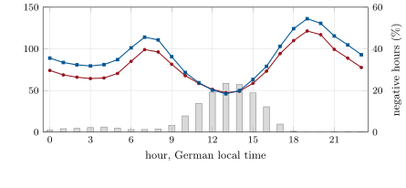
Germany’s prices have the shape a battery needs (Figure 23.1): cheap at midday when solar peaks, dear in the evening. Prices were negative in 457 hours in 2024 and 573 in 2025, down to $-$ € 250.32; at 13:00 local time 23.4% of hours were negative, and at 19:00 none. The battery is scheduled each day by dynamic programming over its state of charge and the energy charged so far (Listing 23.2), with a round-trip efficiency of 88% and one full cycle a day. On the 727 days with 24 hours, knowing each day’s auction prices in advance, as in Book 3, it earns € 69 900 per MW a year. A quarter of its charging hours (24.8%) have negative prices.

Figure 23.1. German day-ahead prices (DE-LU) by hour of the day, averaged over 2024 and over 2025, and the share of hours with negative prices over both years. Data: Bundesnetzagentur / SMARD.de (CC BY 4.0).

The battery that has sold its day-ahead schedule can change it intraday: buy back power it no longer wants to deliver, or sell more, paying the half-spread on every MWh it changes. Re-optimising against the day’s intraday prices, the schedule changes on 71% of days:

1 MW, 2 MWh, 88% round trip	day-ahead (€ a year)	intraday extra (€ a year)
one cycle a day, half-spread € 1	69 900	2 900
one cycle, no spread	69 900	3 800
one cycle, half-spread € 3	69 900	1 600
two cycles a day, half-spread € 1	83 800	4 900

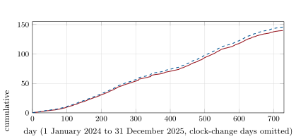
Both columns are generous. The day-ahead column knows the auction’s prices before bidding into it; the intraday column re-optimises once with the whole day’s intraday prices known. The intraday extra is small because the planted errors move prices by a few euros, while the day’s price range averaged over a hundred (Figure 23.2).

Cumulative revenue of a 1 MW, 2 MWh battery on German day-ahead prices, 2024–2025, and with its schedule re-optimised against synthetic intraday prices. Data: Bundesnetzagentur / SMARD.de (CC BY 4.0); s2_powergas.battery_table. — **Figure 23.2.** Cumulative revenue of a 1 MW, 2 MWh battery on German day-ahead prices, 2024–2025, and with its schedule re-optimised against synthetic intraday prices. Data: Bundesnetzagentur / SMARD.de (CC BY 4.0); `s2_powergas.battery_table`.

23.4 Risk in power books

Power cannot be stored in bulk, so every hour is its own product, and a power book is a book of 8 760 contracts a year, each with its own weather. Its risks are the forecast errors themselves, which are correlated across hours (a wrong wind forecast is wrong all afternoon); prices that jump by hundreds of euros when a few gigawatts go missing (the 2024 maximum was € 936.28); imbalance charges for delivering less than sold (Book 3, chapter 6); and the limits of the physical asset, a battery that is full when prices go negative. A battery also degrades with each cycle, which the table above does not charge. A second cycle a day adds € 13 800 of day-ahead revenue at a cost in battery life that the owner must price.

23.5 Strategy files

Strategy file 23.1 — Forecast-error intraday trade

Who pays you, and why. Generators and suppliers who must balance their forecast errors intraday.

Instruments and venues. Day-ahead auction; continuous intraday market.

Signal. The trader’s forecast of wind, solar and load against the auction’s.

Sizing and execution. Positions scaled to the forecast’s confidence; closed intraday.

Costs. Intraday bid-ask; imbalance charges on what is not closed.

How it dies. Better public forecasts; costs.

Horizon, capacity, infrastructure. Hours; weather models and fast intraday access.

Backtest honestly. Forecasts as of the auction, not later ones.

Sources. Kiesel and Paraschiv (2017); Ziel (2017); this chapter: € 2.54 per MWh at a skill of 0.5.

Strategy file 23.2 — Weather-driven gas position

Who pays you, and why. Market participants who price yesterday’s forecast.

Instruments and venues. Gas futures for the next weeks; power baseload.

Signal. Revisions of heating and cooling degree-day forecasts against the priced forecast.

Sizing and execution. In proportion to the revision’s expected demand effect.

Costs. Futures bid-ask.

How it dies. Everyone has the same models; revisions priced in minutes.

Horizon, capacity, infrastructure. Days to weeks.

Backtest honestly. Forecast vintages as issued.

Sources. No performance figure verified.

Strategy file 23.3 — Battery day-ahead arbitrage

Who pays you, and why. The daily price shape: solar at midday, demand in the evening.

Instruments and venues. A battery; day-ahead auction; intraday market; reserves.

Signal. Forecast day-ahead prices; then intraday prices.

Sizing and execution. A daily schedule by dynamic programming; re-optimised intraday.

Costs. Round-trip losses; degradation; spreads.

How it dies. More batteries flattening the shape.

Horizon, capacity, infrastructure. Hours; the asset.

Backtest honestly. Price forecasts, not realised auction prices; degradation per cycle.

Sources. This chapter: € 69 900 per MW a year day-ahead with foresight, € 2 900 more intraday.

Strategy file 23.4 — Spark-spread plant optimisation

Who pays you, and why. The spread between power and fuel in the hours a plant runs.

Instruments and venues. A gas plant or a tolling contract; power, gas and carbon forwards.

Signal. The clean spark spread by hour against the plant’s costs.

Sizing and execution. Dispatch when the spread exceeds costs; hedge forward in blocks.

Costs. Start-up costs; minimum run times.

How it dies. Renewables that take the plant’s hours.

Horizon, capacity, infrastructure. Hours to years.

Backtest honestly. Start-up and ramping constraints.

Sources. No performance figure verified.

Strategy file 23.5 — Negative-price hours

Who pays you, and why. Producers who must or will run at any price (subsidy schemes, inflexible plants).

Instruments and venues. Flexible load or storage; day-ahead and intraday markets.

Signal. Forecast solar and wind against load at midday and on holidays.

Sizing and execution. Consume or charge in negative hours.

Costs. Network charges on consumption.

How it dies. Subsidy rules that stop paying in negative hours; more flexible demand.

Horizon, capacity, infrastructure. Hours.

Backtest honestly. Network charges; the forecast, not the realised price.

Sources. SMARD data: 457 negative hours in 2024 and 573 in 2025.

23.6 Tutorial: the wind forecast

Goal. Measure the German price profile and negative hours, simulate intraday prices from wind forecast errors, trade the errors, and schedule a battery day-ahead and then intraday. End state: the three tables and two figures.

Intraday prices and the forecast trade.

def intraday(da: np.ndarray, cfg: PowerConfig | None = None) -> tuple[np.ndarray, np.ndarray]:
    cfg = cfg or PowerConfig()
    rng = np.random.default_rng(cfg.seed)
    days = da.shape[0]
    err = np.empty((days, 24))
    err[:, 0] = cfg.err_sd * rng.standard_normal(days)
    step = cfg.err_sd * math.sqrt(1 - cfg.err_phi ** 2)
    for h in range(1, 24):
        err[:, h] = cfg.err_phi * err[:, h - 1] + step * rng.standard_normal(days)
    idp = da - cfg.beta * err + cfg.id_noise * rng.standard_normal((days, 24))
    return idp, err


def forecast_trade(da: np.ndarray, idp: np.ndarray, err: np.ndarray, cfg: PowerConfig | None = None) -> dict:
    """Sell 1 MWh day-ahead and buy it back intraday when the forecast says more wind than the auction assumed; the
    reverse when less; nothing when the forecast is small. P&L per hour in EUR."""
    cfg = cfg or PowerConfig()
    rng = np.random.default_rng(cfg.seed + 1)
    signal = cfg.skill * err / cfg.err_sd + math.sqrt(1 - cfg.skill ** 2) * rng.standard_normal(err.shape)
    pos = np.where(signal > cfg.threshold, -1.0, np.where(signal < -cfg.threshold, 1.0, 0.0))   # + buys day-ahead
    pnl = pos * (idp - da) - cfg.id_cost * np.abs(pos)
    return {"pnl": pnl, "pos": pos, "ic": float(np.corrcoef(signal.ravel(), (da - idp).ravel())[0, 1])}

Listing 23.1. Wind errors move intraday prices; a partial forecast trades them. code/firm/powergas/firm_powergas.py

The battery.

def battery(prices: np.ndarray, cfg: PowerConfig | None = None, committed: np.ndarray | None = None) -> dict:
    """Schedule each day by dynamic programming over (state of charge, energy charged so far). Charging one MWh into
    the battery buys 1/sqrt(eff) MWh from the grid; discharging one sells sqrt(eff). Without `committed`, cash is
    -price x grid MWh. With `committed` (a schedule already sold day-ahead), cash is the cost of changing it at these
    prices: -price x (new - committed) - id_cost x |new - committed|."""
    cfg = cfg or PowerConfig()
    days = prices.shape[0]
    e, cmax = cfg.energy, cfg.energy * cfg.cycles
    grid = {1: 1 / math.sqrt(cfg.eff), 0: 0.0, -1: -math.sqrt(cfg.eff)}          # grid MWh per step of charge
    old = np.zeros_like(prices) if committed is None else committed
    cost = 0.0 if committed is None else cfg.id_cost
    V = np.full((days, e + 1, cmax + 1), -np.inf)
    V[:, 0, :] = 0.0                                                          # end empty
    policy = []
    for h in range(23, -1, -1):
        W, A = np.full_like(V, -np.inf), np.zeros(V.shape, int)
        for s in range(e + 1):
            for c in range(cmax + 1):
                for a in (-1, 0, 1):
                    s2, c2 = s + a * cfg.power, c + max(a, 0) * cfg.power
                    if not (0 <= s2 <= e and c2 <= cmax):
                        continue
                    g = grid[a] * cfg.power
                    v = -prices[:, h] * (g - old[:, h]) - cost * np.abs(g - old[:, h]) + V[:, s2, c2]
                    better = v > W[:, s, c]
                    W[:, s, c], A[:, s, c] = np.where(better, v, W[:, s, c]), np.where(better, a, A[:, s, c])
        V = W
        policy.append(A)
    policy.reverse()
    sched = np.zeros_like(prices)
    s, c, idx = np.zeros(days, int), np.zeros(days, int), np.arange(days)
    for h in range(24):
        a = policy[h][idx, s, c]
        sched[:, h] = np.vectorize(grid.get)(a) * cfg.power
        s, c = s + a * cfg.power, c + np.maximum(a, 0) * cfg.power
    return {"grid": sched, "cash": V[:, 0, 0]}

Listing 23.2. Daily dynamic programming, day-ahead or against a committed schedule. code/firm/powergas/firm_powergas.py

Run real(), trade(), battery_table() and fig_powergas.py.

What to change next. Bid the battery on a price forecast instead of the auction’s prices; re-optimise intraday hour by hour; add a degradation cost per cycle.

23.7 Build: power and gas

Purpose. Intraday prices from forecast errors, the forecast-error trade, and battery scheduling day-ahead and intraday.

Interface. PowerConfig(…), intraday(da, cfg), forecast_trade(da, idp, err, cfg), battery(prices, cfg, committed).

Rules. Charging costs $1/\sqrt{\eta}$ of the grid energy, discharging returns $\sqrt{\eta}$ ; the battery ends each day empty; deviations from a committed schedule pay the half-spread.

Acceptance tests. code/firm/powergas/tests/: no errors, no spread; a perfect forecast never loses without costs; the battery by hand; re-optimising on the committed prices changes nothing.

Stretch. Quarter-hour products; reserves; degradation.

Sources and further reading

R. Kiesel and F. Paraschiv, “Econometric analysis of 15-minute intraday electricity prices”, Energy Economics 64, 2017.
F. Ziel, “Modeling the impact of wind and solar power forecasting errors on intraday electricity prices”, 14th International Conference on the European Energy Market, 2017.
Bundesnetzagentur / SMARD.de, hourly day-ahead prices, generation and load for Germany, 2024–2025, CC BY 4.0 (Book 3’s file).

23.8 Exercises

Exercise 23.1 ★

Wind comes in 1.5 GW above the auction’s forecast. At € 3.05 per MWh per GW, how far should the intraday price be below the day-ahead price?

Solution

Solution of Exercise 23.1.

$1.5 \times 3.05 = 4.575$ : about € 4.6 per MWh below the day-ahead price, before other noise.

Exercise 23.2 ★

A battery buys 2 MWh of storage at € 0 and sells it at € 100 with a round-trip efficiency of 88%. What does it earn?

Solution

Solution of Exercise 23.2.

Charging 2 MWh of storage at € 0 costs nothing; discharging returns $2\sqrt{0.88} = 1.876$ MWh to the grid (the charging side lost the other $\sqrt{0.88}$ factor, paid at € 0), sold at € 100: € 187.62.

Exercise 23.3 ★

The forecast trade earns € 2.54 per MWh on 61% of hours with 1 MW. Check the annual figure over two years of 727 days.

Solution

Solution of Exercise 23.3.

$2.54 \times 0.61 \times 24 \times 727 / 2 \approx 13\,500$ : about € 13 500 a year; with unrounded inputs, € 13 600.

Exercise 23.4 ★★

Why does the forecast trade’s edge fall so fast with a half-spread of € 3?

Solution

Solution of Exercise 23.4.

The edge is about € 3.5 per MWh before costs (€ 2.54 after a € 1 half-spread); a € 3 half-spread takes most of it, leaving € 0.54. A forecast edge measured in a few euros is small against costs of a few euros.

Exercise 23.5 ★★

Why are German prices most often negative at midday?

Solution

Solution of Exercise 23.5.

Solar output peaks at midday; when it and wind exceed demand plus export capacity, producers that must or will run regardless (subsidised output, inflexible plants) bid below zero. In 2024–2025, 23.4% of hours at 13:00 were negative, none at 19:00.

Exercise 23.6 ★★

Kiesel and Paraschiv found an asymmetric response to forecast errors; Ziel found none significant. How could both be right?

Solution

Solution of Exercise 23.6.

They asked different questions with different data and models: Kiesel and Paraschiv let the response depend on a threshold in the expected demand covered by conventional capacity, so the asymmetry can appear only in some states; Ziel tested whether positive and negative errors differ within his model and found no significant difference. An effect that exists only above a threshold can vanish in an average.

Exercise 23.7 ★★★

Coding. Run battery_table(PowerConfig(cycles=2)). What does the second cycle add, and what does the table leave out?

Solution

Solution of Exercise 23.7.

Day-ahead revenue rises from € 69 900 to € 83 800, € 13 800 more, and the intraday extra from € 2 900 to € 4 900. The table leaves out degradation: each extra cycle uses up battery life, and the second cycle of the day uses the smaller price differences.

Exercise 23.8 ★★★

Find the flaw. “Our battery backtest earned € 69 900 per MW a year on German day-ahead prices; that is what we will earn.”

Solution

Solution of Exercise 23.8.

The backtest scheduled each day knowing that day’s auction prices, which a real operator must forecast before bidding; it charged no degradation, no bid-ask and no network charges. It is an upper bound for the day-ahead market alone, not a forecast; intraday and reserve revenues, which it omits, push the other way.

23.9 Problem: The Wind Forecast

Problem 23.1

Weekend problem — power and gas trading

Germany’s day-ahead prices, the synthetic intraday market and the public record.

Part I — The markets.

Define the day-ahead-intraday spread.
Give the slope and correlation of price on residual load.
How are the synthetic intraday prices built, and what is planted?
What did Kiesel and Paraschiv and Ziel find?

Part II — The forecast trade.

Describe the trade.
Give its results at each skill and cost.
Define a weather-driven position.
How does the trade die?

Part III — The battery.

Define battery arbitrage.
Describe the price profile and negative hours.
How is the battery scheduled?
Give the battery table.

Part IV — The verdict.

State the named result: the battery’s revenue in day-ahead only and with intraday re-optimisation.
Why are both columns generous?
Why is the intraday extra small here?
What are the risks of a power book?
How would you backtest the battery honestly?
Which strategy file dies first as batteries multiply?
How does the forecast trade relate to chapter 15’s flow trades?
In one sentence: what does a power trader sell?

Solution

Solution of Problem 23.1.

The day-ahead price less the intraday price for the same hour, driven by what changed between the auction and delivery.
€ 3.05 per MWh per GW of residual load, correlation 0.83, over 2024–2025.
The day-ahead price less € 3.05 per GW of unexpected wind, errors of 2 GW standard deviation with hourly autocorrelation 0.9, plus € 6 of noise; all of it planted.
Kiesel and Paraschiv: intraday prices adjust asymmetrically to renewable forecast errors and volume, depending on a demand threshold. Ziel: no significant difference between the effects of positive and negative errors.
Sell day-ahead and buy back intraday when expecting more wind than the auction assumed; the reverse when less; nothing on small forecasts.
Skill 0.5, half-spread € 1: € 2.54 per MWh, € 13 600 a year per MW, IC 0.36; skill 0.3: € 1.08, € 5 800, 0.21; half-spread € 3: € 0.54, € 2 900.
A position in power or gas on a weather forecast that differs from the market’s, closed when forecasts converge or the weather arrives.
Better public forecasts and costs.
Scheduling a battery to charge cheap and discharge dear, day-ahead then intraday, within its limits.
Cheap at midday, dear in the evening; 457 negative hours in 2024 and 573 in 2025, 23.4% of hours at 13:00.
Daily dynamic programming over state of charge and energy charged, one cycle, 88% round trip, ending empty.
Day-ahead € 69 900 a year; intraday extra € 2 900 (€ 3 800 without spread, € 1 600 at € 3); two cycles € 83 800 and € 4 900.
€ 69 900 per MW a year day-ahead, € 72 800 with intraday re-optimisation (€ 2 900 more), on 2024–2025 German prices.
The day-ahead schedule knows the auction’s prices; the intraday one knows the day’s intraday prices at once.
The planted errors move prices by a few euros, while the daily range averages over a hundred.
Correlated forecast errors across hours, price jumps, imbalance charges, the asset’s limits and degradation.
Bid on price forecasts made before the auction, re-optimise intraday as prices arrive, and charge degradation and fees.
Battery day-ahead arbitrage: more batteries flatten the daily shape it trades.
Both are paid by participants who must trade (flows at a fix, generators balancing errors), and both need a forecast of that need.
Delivery at a particular hour, and the information about what that hour will need.

23.10 Interview questions

Interview question 23.1 ★ trader

Why can power prices be negative?

Solution

Solution of Interview question 23.1.

Some producers are paid to produce (subsidies per MWh) or cannot stop cheaply (inflexible plants), so they bid below zero rather than cut output; when their supply exceeds demand and export capacity, the auction clears below zero.

Interview question 23.2 ★★ researcher

How would you forecast the day-ahead-intraday spread for tomorrow’s hours?

Solution

Solution of Interview question 23.2.

Forecast the change in wind, solar and load between the auction’s forecasts and one’s own, translate it to price through the residual-load slope in that hour’s state of the merit order, and check against realised spreads; include plant outages and interconnector flows.

Interview question 23.3 ★★ trader

Your wind forecast is 3 GW above the market’s for tomorrow afternoon. What do you do, and how much?

Solution

Solution of Interview question 23.3.

Sell those hours day-ahead and plan to buy back intraday, sized by the forecast’s track record at that lead time and the expected price effect (about € 3 per GW here), and within limits for correlated errors across the afternoon’s hours.

Interview question 23.4 ★★ risk

How would you set limits for an intraday power desk?

Solution

Solution of Interview question 23.4.

Limits on open position by hour and by block, on the sum of correlated hours, on imbalance exposure at gate closure, on loss per day, and stress tests for price spikes and forecast failures.

Interview question 23.5 ★★ developer

Design the system that schedules a fleet of batteries every quarter hour.

Solution

Solution of Interview question 23.5.

A price-forecast service; an optimiser per battery (dynamic programming or a linear programme) re-run on each new price; a position keeper that nets the fleet against markets; order routing to the intraday market; telemetry of state of charge and availability; and a fallback schedule.

Interview question 23.6 ★★★ researcher

A battery with round-trip efficiency $\eta$ buys at $p_1$ and sells at $p_2$ . Show that the trade pays only if $p_2 > p_1/\eta$ (for positive prices), and say what changes when $p_1 < 0$ .

Solution

Solution of Interview question 23.6.

Buying 1 MWh at $p_1$ returns $\eta$ MWh sold at $p_2$ : profit $\eta p_2 - p_1 > 0$ iff $p_2 > p_1/\eta$ . With $p_1 < 0$ the battery is paid to charge, so the trade pays whenever $\eta p_2 > p_1$ , including some negative $p_2$ ; the constraint then is capacity, not price.

Terms defined in this chapter

See all 2333 terms in the glossary