Strategies II: Volatility, Relative Value, Macro and the Bank Desks · Strategies

2Dispersion and Correlation

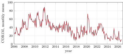
An index option is a bet on the index’s volatility, which depends on how volatile its members are and how much they move together. Cboe publishes the correlation that option prices imply among the 50 largest S&P 500 stocks: from 2006 to 2026 it averaged 37, reached 96.6 on 24 October 2008, and fell to 2.93 in July 2024. Driessen, Maenhout and Vilkov found that correlation risk is priced: selling it, by selling index volatility against members’ volatility, earned a high alpha before frictions and none after them. On this chapter’s synthetic market the same trade earns a Sharpe ratio of 0.65 made vega-neutral, and a pure short correlation swap 1.74, until a crash takes correlation from 0.12 to 0.83 in a month. The build is firm.dispersion.

2.1 Index volatility from member volatilities

An index’s variance is the weighted sum of its members’ variances and covariances: $\sigma_I^2 = \sum_i w_i^2\sigma_i^2 + \sum_{i \ne j} w_i w_j \rho_{ij}\sigma_i\sigma_j$ . Replacing every pairwise correlation by one average $\bar\rho$ and solving gives the average correlation that makes the members’ volatilities consistent with the index’s:

\bar\rho = \frac{\sigma_I^2 - \sum_i w_i^2\sigma_i^2}{\sum_{i \ne j} w_i w_j \sigma_i\sigma_j}.

Cboe’s implied correlation indices apply this decomposition to the implied volatilities of the S&P 500 and of its 50 largest members.

Definition 2.1 (Realised correlation)

Realised correlation is the average correlation among an index’s members computed from realised variances over a period with the same decomposition as implied correlation: the index’s realised variance against the members’ realised variances.

firm.dispersion (Listing 2.1) computes both. On the synthetic market the index is the equal-weighted average of thirty members; members’ implied variance is their expected variance times 1.10 and the index’s times 1.30, so the index’s options are dearer than its members’ and implied correlation sits above what follows: 0.311 on average against a realised 0.252, higher in 77% of months.

2.2 The correlation risk premium

Definition 2.2 (Correlation risk premium)

The correlation risk premium is the difference between the average correlation implied by index and member option prices and the correlation then realised; it is positive on average because correlation rises in crashes, when diversification is most needed.

Driessen, Maenhout and Vilkov used S&P 100 index options and options on all its components: correlation risk was priced, it explained the cross-section of index and single-stock option returns, and a strategy selling it had a high alpha for an investor without frictions. With realistic trading costs the premium could not be exploited, which they read as a limit to arbitrage. Cboe’s own comparison with a smoothed realised correlation of the top 50 stocks finds realised usually slightly below implied.

The real index (Figure 2.1) shows why selling correlation is uncomfortable: COR1M averaged 37.0 from January 2006 to September 2026, with 5% and 95% quantiles of 10.8 and 69.7, and averaged 70.4 in October 2008 and 72.5 in March 2020. On 22 September 2026 it stood at 7.59; its low was 2.93, on 12 July 2024. Cboe’s S&P 500 dispersion index, published since June 2014, averaged 25.5 and peaked at 58.9 on 18 March 2020.

Cboe’s 1-Month Implied Correlation Index (the average correlation among the S&P 500’s 50 largest members implied by index and single-stock options), monthly means, January 2006 to September 2026. Derived from Cboe’s index history; the raw series is not redistributed. Data: s2_fetch_cor. — **Figure 2.1.** Cboe’s 1-Month Implied Correlation Index (the average correlation among the S&P 500’s 50 largest members implied by index and single-stock options), monthly means, January 2006 to September 2026. Derived from Cboe’s index history; the raw series is not redistributed. Data: `s2_fetch_cor`.

2.3 Dispersion trades and their weights

A dispersion trade (Book 5, chapter 17) sells index volatility and buys members’ volatility. The chapter’s books use one-month variance swaps, rebuilt monthly (Listing 2.2): short one unit of index variance, long members’ variance on notionals set one of two ways.

Definition 2.3 (Dispersion weighting)

Dispersion weighting is the choice of the members’ notionals in a dispersion trade: equal to their index weights, so that the trade is short correlation and long the members’ specific variance; or scaled so that the members’ total vega equals the index’s (vega-neutral), so that a common rise in volatility leaves the book flat and its P&L comes mainly from correlation.

239 months	Sharpe ratio	skewness	worst month (sd)	months up
members on index weights	$-0.02$	2.67	$-1.6$	36%
vega-neutral	0.65	$-5.87$	$-11.3$	70%
short correlation swap	1.74	$-1.67$	$-6.0$	77%

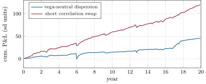
On index weights the book is long more member variance than it is short index variance, and it pays the members’ own premium: it loses a little on average and gains in crashes (positive skewness). Made vega-neutral it earns the correlation premium with the familiar short-volatility shape. The correlation swap, which pays implied minus realised correlation directly, isolates the premium best; its Sharpe ratio is the highest and its worst month is still six standard deviations.

2.4 When correlation goes to one

The three planted crashes are the tests (Figure 2.2). In the first, implied correlation was 0.12 when the month began and realised correlation 0.83: the vega-neutral book lost 11.3 of its monthly standard deviations and the correlation swap 0.71 of a unit. In the second, 0.12 against 0.57 (3.0 standard deviations and 0.45). In the third, which began when implied correlation was already 0.73, the loss was under one standard deviation. A crash is a correlation event: every member falls together, the index falls as far as its members, and the diversification the index option was priced to lack arrives.

The synthetic vega-neutral dispersion book and short correlation swap, each cumulated in units of its monthly standard deviation, over twenty years with crashes at years 6.0, 12.7 and 17.5. Data: s2_dispersion.monthly. — **Figure 2.2.** The synthetic vega-neutral dispersion book and short correlation swap, each cumulated in units of its monthly standard deviation, over twenty years with crashes at years 6.0, 12.7 and 17.5. Data: `s2_dispersion.monthly`.

2.5 Strategy files

Strategy file 2.1 — Vega-weighted dispersion

Who pays you, and why. Buyers of index protection, who pay for the correlation that crashes bring.

Instruments and venues. Index options or variance swaps against single-stock options or variance swaps on the largest members.

Signal. Implied against forecast correlation.

Sizing and execution. Members’ vega matched to the index’s; monthly or quarterly rolls; members limited to liquid names.

Costs. Single-stock option spreads, the main friction.

How it dies. Crashes; frictions that absorb the premium.

Horizon, capacity, infrastructure. Months; single-stock surfaces for dozens of names.

Backtest honestly. Single-stock option costs; crash months in the sample.

Sources. Driessen, Maenhout and Vilkov (2009); this chapter: 0.65 and an 11-standard-deviation crash month.

Strategy file 2.2 — Theta-weighted dispersion

Who pays you, and why. As for vega-weighted dispersion.

Instruments and venues. Index and single-stock straddles.

Signal. As above.

Sizing and execution. Members’ theta matched to the index’s, so that the book’s time decay is neutral and its P&L is gamma against gamma.

Costs. Delta hedging of many options.

How it dies. As above.

Horizon, capacity, infrastructure. Weeks to months; a hedging engine.

Backtest honestly. Hedging costs for every member.

Sources. No performance figure verified.

Strategy file 2.3 — Correlation swap short

Who pays you, and why. Buyers of correlation protection, often structured-product desks (chapter 28).

Instruments and venues. Over-the-counter correlation swaps.

Signal. Strike against forecast correlation.

Sizing and execution. Sized by the crash-month loss.

Costs. Dealer spreads; counterparty exposure.

How it dies. Crashes.

Horizon, capacity, infrastructure. Months to a year; an over-the-counter relationship.

Backtest honestly. Realised correlation measured as the contract defines it.

Sources. This chapter: 1.74 before costs, a loss of 0.71 of a unit in the first crash.

Strategy file 2.4 — Sector dispersion

Who pays you, and why. As for index dispersion, within a sector.

Instruments and venues. Sector ETF options against their largest members’ options.

Signal. Sector implied correlation against its history.

Sizing and execution. Vega-neutral within sectors.

Costs. Wider spreads on sector options.

How it dies. Sector-wide shocks.

Horizon, capacity, infrastructure. Months; small capacity.

Backtest honestly. Liquidity of sector options.

Sources. Cboe’s sector implied correlations (as a data source); no performance figure verified.

2.6 Tutorial: when everything moves together

Goal. Measure implied and realised correlation on the synthetic index and its members, run three dispersion books through the planted crashes, and read Cboe’s correlation and dispersion indices. End state: the table and the two figures.

Correlation and the legs.

def average_corr(var_index, var_members, w):
    var_members, w = np.asarray(var_members, float), np.asarray(w, float)
    vol = np.sqrt(var_members)
    own = (w**2 * var_members).sum(-1)
    cross = (w * vol).sum(-1) ** 2 - own
    return (np.asarray(var_index, float) - own) / cross


def realised_var(R, start: int, n: int, year: int = 252):
    x = np.asarray(R, float)[start + 1:start + 1 + n]
    return (x**2).sum(0) * year / n


def dispersion_pnl(iv_index, iv_members, rv_index, rv_members, w, vega_neutral: bool = False):
    """Variance-swap legs in annual variance units (multiply by the period's length for P&L). A variance swap on
    notional n has vega 2 n iv; with vega_neutral the members' notionals n_i = c w_i are scaled so that
    sum_i n_i iv_i = iv_index, otherwise n_i = w_i."""
    w, iv_m = np.asarray(w, float), np.asarray(iv_members, float)
    iv_i = np.asarray(iv_index, float)
    n = w * (iv_i / (w * iv_m).sum(-1))[..., None] if vega_neutral else w
    index_leg = iv_i**2 - np.asarray(rv_index, float)
    member_leg = (n * (np.asarray(rv_members, float) - iv_m**2)).sum(-1)
    return index_leg + member_leg


def corr_swap_pnl(implied, realised):
    return np.asarray(implied, float) - np.asarray(realised, float)

Listing 2.1. Average correlation, realised variance and the dispersion P&L. code/firm/dispersion/firm_dispersion.py

The monthly books.

def monthly(member_vrp: float = 0.10):
    cfg = VolConfig(member_vrp=member_vrp)
    S = simulate_vol(cfg)
    R, spec = S["R"], S["spec"]
    N = R.shape[1]
    w = np.full(N, 1 / N)
    idx = R @ w
    tau = TENOR / 252
    out = {k: [] for k in ("ic", "rc", "weights", "vega", "corrswap", "start")}
    for s in periods(len(idx), TENOR):
        ev = expected_var(S["v"][s], cfg, tau)
        ivm = np.sqrt((ev + spec**2) * (1 + cfg.member_vrp))
        ivi = math.sqrt((ev + (w**2 * spec**2).sum()) * (1 + cfg.vrp))
        rvi, rvm = realised_var(idx[:, None], s, TENOR)[0], realised_var(R, s, TENOR)
        ic, rc = average_corr(ivi**2, ivm**2, w), average_corr(rvi, rvm, w)
        out["ic"].append(ic)
        out["rc"].append(rc)
        out["weights"].append(dispersion_pnl(ivi, ivm, rvi, rvm, w, False) * tau)
        out["vega"].append(dispersion_pnl(ivi, ivm, rvi, rvm, w, True) * tau)
        out["corrswap"].append(corr_swap_pnl(ic, rc))
        out["start"].append(s)
    out = {k: np.array(v, float) for k, v in out.items()}
    out["crash_periods"] = [s // TENOR for s, _ in S["crashes"]]
    return out

Listing 2.2. Implied and realised correlation and three books, month by month. code/strategies-2/02-dispersion-and-correlation/python/s2_dispersion.py

Run s2_fetch_cor.py once, then monthly(), crashes() and fig_dispersion.py.

What to change next. Trade only the twenty largest members and measure the tracking of the index; add a correlation skew so that crash correlation is priced; hedge the vega-neutral book with a small long correlation position before calm periods end.

2.7 Build: dispersion

Purpose. Implied and realised average correlation, dispersion books on variance swaps and correlation swaps.

Interface. average_corr(var_index, var_members, w), realised_var(R, start, n), dispersion_pnl(iv_index, iv_members, rv_index, rv_members, w, vega_neutral), corr_swap_pnl(implied, realised).

Rules. The same decomposition for implied and realised correlation; variance swap legs in annual variance units.

Acceptance tests. code/firm/dispersion/tests/: a common correlation recovered exactly; zero P&L when every leg realises its implied variance; the vega-neutral notionals by hand.

Stretch. Straddle legs with hedging; correlation skew; sector baskets.

Sources and further reading

J. Driessen, P. J. Maenhout and G. Vilkov, “The price of correlation risk: evidence from equity options”, Journal of Finance 64(3), 2009.
Cboe, S&P 500 Implied Correlation Index methodology and implied correlation notes.
Cboe Global Markets, daily histories of COR1M and DSPX.

2.8 Exercises

Exercise 2.1 ★

An index of many equal-weighted members has implied volatility 20% and each member 30%. What average correlation does that imply?

Solution

Solution of Exercise 2.1.

For many equal-weighted members the own-variance term vanishes and $\bar\rho \approx \sigma_I^2/\sigma^2 = 0.04/0.09 = 0.444$ .

Exercise 2.2 ★

For a vega-neutral dispersion trade with index implied volatility 20% and members at 30%, by what factor are the members’ notionals scaled from their index weights?

Solution

Solution of Exercise 2.2.

By $\sigma_I/\sum_i w_i\sigma_i = 0.2/0.3 = 0.667$ .

Exercise 2.3 ★

Why does the book on index weights have positive skewness?

Solution

Solution of Exercise 2.3.

On index weights the book is long more member variance than it is short index variance, so it gains when volatility rises broadly (crashes) and pays the members’ premium in calm months: small regular losses, rare gains.

Exercise 2.4 ★★

A short correlation swap was struck at 0.12 and correlation realised 0.83. What does it lose per unit, and why did the strike look reasonable when set?

Solution

Solution of Exercise 2.4.

$0.12 - 0.83 = -0.71$ per unit. The strike reflected a calm month’s expectations: implied correlation is low when markets are calm, which is when crashes that raise correlation begin.

Exercise 2.5 ★★

Why could Driessen and co-authors find a priced correlation premium that could not be exploited?

Solution

Solution of Exercise 2.5.

The premium is measured on the index and all members; trading it needs options on every member, whose spreads and hedging costs are large relative to the premium: a limit to arbitrage, which is also why the premium can persist.

Exercise 2.6 ★★

COR1M fell to 2.93 in July 2024. What does a low implied correlation say about index options against single-stock options, and what risk does selling correlation there carry?

Solution

Solution of Exercise 2.6.

Index options are cheap relative to single-stock options: members are expected to move apart. Selling correlation from there has little premium left and a large loss if members start moving together, as they do in a sell-off.

Exercise 2.7 ★★★

Coding. Run monthly(0.30), which sets the members’ premium equal to the index’s. What happens to the correlation premium and the books?

Solution

Solution of Exercise 2.7.

With the members’ premium equal to the index’s, implied correlation averages 0.258 against a realised 0.252: the correlation premium nearly vanishes (0.006). The correlation swap’s Sharpe ratio falls to 0.17, the vega-neutral book loses ( $-1.84$ ), and the book on index weights loses every month ( $-17.3$ ), because it pays the full variance premium on more member variance than it sells on the index.

Exercise 2.8 ★★★

Find the flaw. “Implied correlation has exceeded realised in 77% of months, so a short correlation swap is a high-probability trade we can lever.”

Solution

Solution of Exercise 2.8.

Winning in 77% of months is the shape of a short-volatility trade: the losses come in the others, and the first crash cost the correlation swap six monthly standard deviations. Leverage chosen on the frequency of wins would not survive the size of the losses; size it by a crash-month stress.

2.9 Problem: When Everything Moves Together

Problem 2.1

Weekend problem — selling correlation

The chapter’s synthetic index, Cboe’s indices and the public record.

Part I — Correlation.

Write the average-correlation formula and explain it.
Define realised correlation and the correlation risk premium.
How does Cboe compute its implied correlation index?
What did Driessen, Maenhout and Vilkov find?

Part II — The real indices.

Give COR1M’s average, range and its 2008 and 2020 levels.
What does DSPX measure, and what were its statistics?
Why is a record low in implied correlation not a free trade?
What did Cboe find comparing implied and realised correlation?

Part III — The books.

Define dispersion weighting and describe the two weightings.
Give the three books’ Sharpe ratios and skewness.
Why does the book on index weights lose on average?
Why is the correlation swap the cleanest exposure?

Part IV — The verdict.

State the named result: the dispersion book’s return from the correlation premium and its loss when correlation jumps.
What happened in each of the three crashes?
Why did the third crash cost less?
How would you size a dispersion book?
How would you backtest one honestly?
Which strategy file is most exposed to single-stock option costs?
How does this chapter relate to chapter 1?
In one sentence: what does a dispersion trader sell?

Solution

Solution of Problem 2.1.

$\bar\rho = (\sigma_I^2 - \sum w_i^2\sigma_i^2)/\sum_{i \ne j} w_i w_j\sigma_i\sigma_j$ : the single correlation that reconciles index and member volatilities.
The same formula on realised variances; implied minus realised correlation.
From SPX implied volatility and the implied volatilities of the 50 largest members, with Markowitz’s decomposition.
Correlation risk is priced and explains option returns; a strategy selling it has a high alpha without frictions and none with them.
37.0 on average, 10.8 to 69.7 for the middle 90%, 96.6 at the peak (24 October 2008), 70.4 and 72.5 in October 2008 and March 2020.
Cboe’s S&P 500 dispersion index: 25.5 on average since 2014, 58.9 at the peak on 18 March 2020.
Little premium is left and the loss if correlation rises is large.
A smoothed realised correlation is in most cases slightly below the implied.
Members’ notionals on index weights, or scaled to match the index’s vega.
$-0.02$ , 0.65 and 1.74; skewness 2.67, $-5.87$ and $-1.67$ .
It pays the members’ premium on more variance than it sells.
It pays implied minus realised correlation directly, with no variance-level exposure.
Named result. The vega-neutral dispersion book earns the correlation premium (implied 0.311 against realised 0.252) at a Sharpe ratio of 0.65, and loses 11.3 monthly standard deviations when correlation jumps from 0.12 to 0.83 in the first crash; the correlation swap earns 1.74 and loses 0.71 of a unit.
0.12 to 0.83, 0.12 to 0.57, 0.73 to 0.84.
Implied correlation was already high when it began.
By the loss in a crash month, with correlation going to one.
Single-stock option costs, crash months, realised correlation as the contract defines it.
Vega-weighted dispersion.
Chapter 1 sold volatility; dispersion sells the part of index volatility that comes from correlation.
Insurance against members moving together.

2.10 Interview questions

Interview question 2.1 ★ researcher

What is implied correlation, and how is it computed?

Solution

Solution of Interview question 2.1.

The single average correlation that makes the index’s implied variance equal to the weighted sum of members’ implied variances and covariances: $(\sigma_I^2 - \sum w_i^2\sigma_i^2)/\sum_{i \ne j} w_i w_j\sigma_i\sigma_j$ with implied volatilities.

Interview question 2.2 ★★ trader

Walk through a dispersion trade and the risks it carries.

Solution

Solution of Interview question 2.2.

Sell index options or variance and buy members’ options or variance, weighted by vega, theta or index weights; it earns the correlation premium and loses when members move together; it also carries single-stock event risk, member liquidity and hedging costs.

Interview question 2.3 ★★ researcher

Why might index options be expensive relative to single-stock options?

Solution

Solution of Interview question 2.3.

Index options insure against market-wide falls, when correlation rises and diversification fails; investors pay for that insurance, and index option supply (overwriting) is smaller than demand, while single-stock options are often supplied by overwriters.

Interview question 2.4 ★★ risk

How would you stress a dispersion book?

Solution

Solution of Interview question 2.4.

Apply historical crash months (2008, 2020) and a hypothetical move of implied and realised correlation to one, with members’ volatilities up; check the loss against limits and the liquidity of unwinding the single-stock legs.

Interview question 2.5 ★★ developer

What data does a dispersion desk need every day, and what can go wrong with it?

Solution

Solution of Interview question 2.5.

Index and member option surfaces, index weights and membership changes, corporate events (earnings, mergers) by member, and borrow for hedges; stale single-stock quotes and membership errors distort implied correlation.

Interview question 2.6 ★★★ researcher

For $N$ equal-weighted members with equal volatility $\sigma$ and average correlation $\rho$ , show that the index variance is $\sigma^2(\rho + (1 - \rho)/N)$ , and derive the implied correlation from index and member volatilities for large $N$ .

Solution

Solution of Interview question 2.6.

With $w_i = 1/N$ and equal $\sigma$ , $\sigma_I^2 = \sum_i\sigma^2/N^2 + \sum_{i \ne j}\rho\sigma^2/N^2 = \sigma^2/N + \rho\sigma^2(N - 1)/N = \sigma^2(\rho + (1 - \rho)/N)$ . For large $N$ , $\rho \approx \sigma_I^2/\sigma^2$ .

Terms defined in this chapter

See all 2333 terms in the glossary