Strategies II: Volatility, Relative Value, Macro and the Bank Desks · Strategies

16Systematic Macro

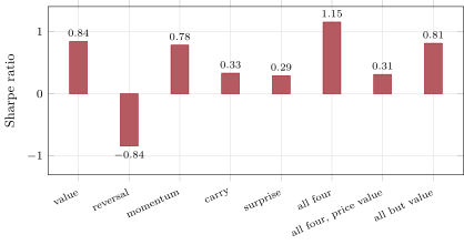
Value, momentum and carry, measured country by country in bonds, currencies and equity indices, make a macro portfolio that no economist designed. Asness, Moskowitz and Pedersen found value and momentum premia in eight markets and asset classes. Each correlated more with its counterparts in other asset classes than the asset classes did with each other, and value and momentum were negatively correlated. On this chapter’s synthetic market of thirty futures, value earns a Sharpe ratio of 0.84, momentum 0.78, carry 0.33 and an economic-surprise signal 0.29. Nearly uncorrelated, they combine to 1.15. Measure value from prices instead of from a fundamental anchor and it becomes momentum’s mirror image, $-0.84$ , and the combination falls to 0.31. The build is firm.sysmacro.

16.1 Signals across countries and assets

The universe is Book 8’s synthetic futures (chapter 19): ten equity indices, ten government bonds and ten currencies, one of each per country, over thirty years, with a persistent drift (the trend) and a carry premium. firm.sysmacro adds two planted effects. Each market carries a valuation gap from fair value with a standard deviation of 10% and a half-life of three years; the price includes the gap, and its reversion is the value premium. Each country has an economic-surprise index with a half-life of 60 days that moves its markets over the following days.

Definition 16.1 (Macro value signal)

A macro value signal ranks countries’ assets by their price against a fundamental anchor, such as purchasing-power parity for a currency, a real-yield or term-premium model for a bond, or earnings and book value for an equity index, buying the cheap and selling the dear.

Each signal is traded long-short within each asset class, reset monthly by rank, and scaled to 10% volatility on its trailing quarter (Listing 16.1). Value uses an anchor that each market’s analyst gets wrong by a persistent 10%. Momentum is the twelve-month return skipping the last month (Book 8, chapter 19), and carry is Book 8’s carry (chapter 20). The price-based variant of value is minus the last five years’ spot move, the return less the carry earned.

16.2 Macro-data signals

Definition 16.2 (Macro momentum)

Macro momentum takes long positions in the assets of countries whose fundamental economic trends (growth, inflation, external balance, monetary policy) are improving and short positions where they are deteriorating, the macro-data counterpart of price momentum.

Definition 16.3 (Economic-surprise signal)

An economic-surprise signal measures how much a country’s recent data releases have exceeded or fallen short of forecasts, and positions its assets for the markets’ delayed response: equities and the currency up and bonds down after positive surprises.

Brooks describes macro momentum as a systematic global macro strategy that is long assets whose macroeconomic trends are improving and short those whose trends are deteriorating, with low correlation to traditional asset classes and diversification in equity bear markets and rising-yield environments. The synthetic surprise signal is a plain version of it. Each country’s index moves its equity index up by 4% a year per unit, its currency up by 3%, and its bond down by 3%, and the trader sees the index with noise of half its size.

16.3 Combining signals

24.5 years, 10% vol each	Sharpe	max drawdown	corr. with momentum
value (anchor)	0.84	$-25\%$	$-0.03$
value from prices (reversal)	$-0.84$		$-0.43$
momentum	0.78	$-23\%$	1
carry	0.33	$-32\%$	0.04
surprise	0.29	$-38\%$	$-0.01$
all four	1.15	$-21\%$
all four, value from prices	0.31
all but value	0.81

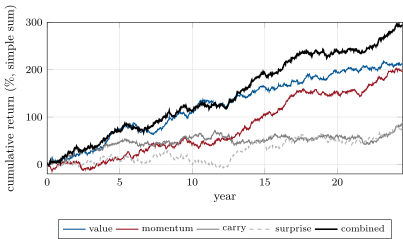
Four nearly uncorrelated signals combine as the arithmetic says. Equal risk budgets give a Sharpe ratio of about the sum of the four divided by the square root of four, 1.12, against 1.15 measured (Figure 16.1). The combination’s worst drawdown, 21%, is smaller than any single signal’s. Value earns its place: without it the combination falls to 0.81.

How value is measured decides whether it helps. In this market the trend lasts about a year, and the last five years’ price move still carries some of it. Minus that move is short the markets that trended up, so the price-based value signal becomes the mirror of momentum: $-0.84$ against 0.78, a correlation of $-0.43$ . Combined, the two cancel, and the four-signal book earns only 0.31. Asness and co-authors found value and momentum both positive and negatively correlated. A synthetic market reproduces that only if value’s anchor is not built from the same prices momentum uses.

Four synthetic macro signals, each scaled to 10% volatility and traded long-short within equities, bonds and currencies, and their equal-risk combination (also at 10%), cumulative sums of daily returns over 24.5 years. Data: s2_sysmacro.books. — **Figure 16.1.** Four synthetic macro signals, each scaled to 10% volatility and traded long-short within equities, bonds and currencies, and their equal-risk combination (also at 10%), cumulative sums of daily returns over 24.5 years. Data: `s2_sysmacro.books`.

16.4 What the record shows

The public record supports the pattern, not the numbers. Asness and co-authors found value and momentum premia everywhere they looked, with a common factor structure across asset classes and a partial link to global funding liquidity. Brooks’s macro momentum adds the trends in economic data. The chapter’s Sharpe ratios are those of a planted market (Figure 16.2). They are there to show how signals combine, not to forecast what a real book would earn. What carries over is the method: measure each signal on its own, measure their correlations, give each a risk budget, and check that value and momentum are not measured from the same data.

Sharpe ratios of the synthetic macro signals and three combinations: all four (value from the anchor), all four with value from prices, and three without value. Data: s2_sysmacro.stats. — **Figure 16.2.** Sharpe ratios of the synthetic macro signals and three combinations: all four (value from the anchor), all four with value from prices, and three without value. Data: `s2_sysmacro.stats`.

16.5 Strategy files

Strategy file 16.1 — Cross-country value

Who pays you, and why. Investors who extrapolate, and a fundamental anchor that prices return to over years.

Instruments and venues. Equity index, bond and currency futures and forwards.

Signal. Price against a fundamental anchor: purchasing-power parity, real yields, earnings yields.

Sizing and execution. Long-short within asset class; monthly; risk-budgeted.

Costs. Futures rolls; low turnover.

How it dies. Anchors that are wrong for years; trends that run further than value can wait.

Horizon, capacity, infrastructure. Years; large capacity.

Backtest honestly. Anchors as they could be computed then, not revised data.

Sources. Asness, Moskowitz and Pedersen (2013); this chapter: 0.84 from an anchor, $-0.84$ from prices.

Strategy file 16.2 — Macro momentum

Who pays you, and why. Markets that price economic news slowly.

Instruments and venues. As above.

Signal. Trends in growth, inflation, external balances and policy; price momentum as a companion.

Sizing and execution. Long-short; monthly.

Costs. Moderate turnover.

How it dies. Turning points; data revisions.

Horizon, capacity, infrastructure. Months; point-in-time macro data.

Backtest honestly. First-release data, not revised.

Sources. Brooks (2017); this chapter: price momentum 0.78.

Strategy file 16.3 — Carry across asset classes

Who pays you, and why. As in Book 8, chapter 20: holders of low-carry assets, and the crash risk of high carry.

Instruments and venues. Futures and forwards in three asset classes.

Signal. Each market’s carry.

Sizing and execution. Long-short within class; risk-budgeted.

Costs. Rolls.

How it dies. Carry crashes.

Horizon, capacity, infrastructure. Months.

Backtest honestly. Carry from futures curves, not assumed rates.

Sources. Book 8, chapter 20; this chapter: 0.33.

Strategy file 16.4 — Economic-surprise tilt

Who pays you, and why. Investors who react slowly to data surprises.

Instruments and venues. Country equity, bond and currency futures.

Signal. Recent releases against consensus forecasts, by country.

Sizing and execution. Long-short; rebalanced as data arrive.

Costs. Higher turnover than value.

How it dies. Forecasters and markets catch up faster.

Horizon, capacity, infrastructure. Weeks to months; a data calendar with forecasts.

Backtest honestly. Release times and first prints.

Sources. This chapter: 0.29; no public performance figure verified.

Strategy file 16.5 — Combined macro factor portfolio

Who pays you, and why. The sum of the above.

Instruments and venues. All of the above.

Signal. Value, momentum, carry and macro data, with equal or estimated risk budgets.

Sizing and execution. Target volatility at the portfolio level.

Costs. Netting reduces turnover.

How it dies. Correlations that rise together in a crisis.

Horizon, capacity, infrastructure. Months; a multi-asset futures book.

Backtest honestly. Signals defined before the test; correlations measured out of sample.

Sources. Asness, Moskowitz and Pedersen (2013); this chapter: 1.15 combined.

16.6 Tutorial: designed by no one

Goal. Plant value and macro-surprise effects in the synthetic futures, build five signals, and combine them. End state: the table and the two figures.

Signals and books.

def signal(m: dict, name: str, t: int):
    lp = m["logp"]
    if name == "value":                                                  # price against a noisy fundamental anchor
        return -m["anchor_gap"][t]
    if name == "reversal":                                               # value from prices: minus the 5-year spot move
        return -(m["spot"][t] - m["spot"][t - 5 * YEAR])
    if name == "momentum":
        return lp[t - 21] - lp[t - YEAR]
    if name == "carry":
        return m["carry"][t]
    return m["seen"][t, m["country"]]


def _within_class(x, cls):
    """Cross-sectional ranks within each class, centred and scaled to unit gross exposure per class."""
    w = np.zeros_like(x, dtype=float)
    for c in np.unique(cls):
        idx = np.where(cls == c)[0]
        rk = np.argsort(np.argsort(x[idx])).astype(float)
        rk -= rk.mean()
        w[idx] = rk / np.abs(rk).sum()
    return w


def portfolio(m: dict, name: str, cfg: MacroConfig | None = None) -> np.ndarray:
    cfg = cfg or MacroConfig()
    r = m["r"]
    T, N = r.shape
    start = 5 * YEAR + 1
    raw = np.zeros(T)
    w = np.zeros(N)
    for t in range(start, T):
        if (t - start) % cfg.every == 0:
            w = _within_class(signal(m, name, t - 1), m["cls"])
        raw[t] = w @ r[t]
    out = np.zeros(T)
    for t in range(start + cfg.lookback, T):
        vol = raw[t - cfg.lookback:t].std() * math.sqrt(YEAR)
        out[t] = raw[t] * (cfg.target_vol / vol if vol > 0 else 0.0)
    return out

Listing 16.1. The five signals, the within-class long-short weights and the vol-targeted book. code/firm/sysmacro/firm_sysmacro.py

The combinations.

@functools.lru_cache(maxsize=1)
def books():
    cfg = MacroConfig()
    m = macro_market(cfg)
    b = {n: portfolio(m, n, cfg) for n in SIGNALS}
    b["combined"] = combine([b[k] for k in ("value", "momentum", "carry", "surprise")], cfg)
    b["combined, price value"] = combine([b[k] for k in ("reversal", "momentum", "carry", "surprise")], cfg)
    b["combined, no value"] = combine([b[k] for k in ("momentum", "carry", "surprise")], cfg)
    return cfg, m, b


def stats():
    _, _, b = books()
    out = {}
    for k, x in b.items():
        x = x[START:]
        cum = np.cumsum(x)
        d = x - x.mean()
        out[k] = {"sr": float(x.mean() / x.std() * math.sqrt(YEAR)), "vol": float(x.std() * math.sqrt(YEAR)),
                  "skew": float((d**3).mean() / (d**2).mean() ** 1.5),
                  "max_dd": float((cum - np.maximum.accumulate(cum)).min())}
    return out

Listing 16.2. Each signal, three combinations, and their statistics. code/strategies-2/16-systematic-macro/python/s2_sysmacro.py

Run stats(), correlations() and fig_sysmacro.py.

What to change next. Estimate risk budgets from trailing correlations instead of equal budgets; add a slow-moving anchor error that drifts; test the price-based value on a market whose trend lasts three months.

16.7 Build: systematic macro

Purpose. Cross-asset value, momentum, carry and macro-surprise signals, and their risk-budgeted combination.

Interface. MacroConfig(…), macro_market(cfg), signal(m, name, t), portfolio(m, name, cfg), combine(books, cfg).

Rules. Signals from data up to the day before; long-short within each class; each book scaled on its own trailing volatility.

Acceptance tests. code/firm/sysmacro/tests/: within-class weights are neutral with unit gross; the market’s shapes and signals; the combination targets its volatility.

Stretch. Estimated risk budgets; real macro data; transaction costs.

Sources and further reading

C. S. Asness, T. J. Moskowitz and L. H. Pedersen, “Value and momentum everywhere”, Journal of Finance 68(3), 2013.
J. Brooks, “A half century of macro momentum”, AQR white paper, 2017.

16.8 Exercises

Exercise 16.1 ★

Four uncorrelated signals have Sharpe ratios of 0.84, 0.78, 0.33 and 0.29 and equal risk budgets. What Sharpe ratio does their combination have?

Solution

Solution of Exercise 16.1.

$(0.84 + 0.78 + 0.33 + 0.29)/\sqrt4 = 1.12$ .

Exercise 16.2 ★

Two signals have Sharpe ratios of 0.84 and 0.78 and a correlation of $-0.43$ . What is the Sharpe ratio of an equal-risk combination?

Solution

Solution of Exercise 16.2.

$(0.84 + 0.78)/\sqrt{2 + 2 \times (-0.43)} = 1.52$ : a negative correlation raises the combination’s Sharpe ratio above the sum over $\sqrt2$ .

Exercise 16.3 ★

A valuation gap has a half-life of three years. What share of it closes in one year?

Solution

Solution of Exercise 16.3.

$1 - 0.5^{1/3} = 21\%$ .

Exercise 16.4 ★★

Why does value measured from five-year price moves become momentum’s mirror image in this market?

Solution

Solution of Exercise 16.4.

The trend lasts about a year, and the five-year price move still contains the recent part of it: minus that move is short the markets that trended up, the opposite of momentum. The anchor-based signal carries no such overlap.

Exercise 16.5 ★★

Why must a macro-data backtest use first-release data?

Solution

Solution of Exercise 16.5.

Macro data are revised, sometimes heavily; a backtest on revised data uses numbers no one had at the time and overstates the signal.

Exercise 16.6 ★★

Why trade signals long-short within each asset class rather than across them?

Solution

Solution of Exercise 16.6.

Asset classes have different volatilities and common factors; within a class the book is neutral to the class’s own direction and trades only the signal, and each class’s risk can be budgeted separately.

Exercise 16.7 ★★★

Coding. Rerun macro_market with MacroConfig(anchor_noise=0.3). What happens to value, and to the combination?

Solution

Solution of Exercise 16.7.

Value falls from 0.84 to 0.69 and the combination from 1.15 to 1.05: a noisier anchor dilutes value, and the other three signals carry the book.

Exercise 16.8 ★★★

Find the flaw. “Our combination has a Sharpe ratio of 1.15, so we will run it at 30% volatility.”

Solution

Solution of Exercise 16.8.

The Sharpe ratio comes from a planted market and from signals whose correlations may rise together in a crisis; at 30% volatility the combination’s worst drawdown of 21% at 10% volatility would be about 63%. Size on stressed correlations and drawdowns, not on the measured ratio.

16.9 Problem: Designed by No One

Problem 16.1

Weekend problem — a systematic macro book

The chapter’s synthetic futures and the public record.

Part I — Signals.

Define the macro value signal and give three anchors.
Define macro momentum and the economic-surprise signal.
How is each signal traded and scaled?
What did Asness, Moskowitz and Pedersen find?

Part II — The planted market.

Describe the valuation gap and the surprise index.
How does the analyst see each?
Why does the anchor’s error matter?
What did Brooks describe?

Part III — Results.

Give each signal’s Sharpe ratio.
Give the correlations.
Give the three combinations’ Sharpe ratios.
Why does value from prices fail here?

Part IV — The verdict.

State the named result: each signal’s Sharpe ratio and the combination’s, with the correlations that make it work.
What does the arithmetic of uncorrelated signals predict?
What happens to the combination in a crisis?
How would you set risk budgets?
How would you backtest the book honestly?
Which strategy file has the highest turnover?
How does this chapter relate to Book 8’s trend and carry chapters?
In one sentence: why does a combination of simple signals work?

Solution

Solution of Problem 16.1.

Price against a fundamental anchor; purchasing-power parity, real yields, earnings yields.
Long improving macro trends, short deteriorating; data releases against forecasts.
Long-short by rank within each class, monthly, scaled to 10% volatility.
Value and momentum premia everywhere, negatively correlated, with common factors across asset classes.
A gap of 10% sd reverting over three years; a surprise index reverting over 60 days.
The gap through an anchor with a persistent 10% error; the surprise with noise of half its size.
It dilutes the signal: at 30% error value earns 0.69.
Macro momentum: long improving fundamentals, short deteriorating, with low correlation to asset classes.
Value 0.84, reversal $-0.84$ , momentum 0.78, carry 0.33, surprise 0.29.
Near zero except reversal and momentum, $-0.43$ .
1.15 with anchor value, 0.31 with price value, 0.81 without value.
It overlaps with the trend and becomes its mirror.
Named result. Value 0.84, momentum 0.78, carry 0.33 and surprise 0.29, nearly uncorrelated, combine to 1.15 with a smaller drawdown than any; value from prices is momentum’s mirror ( $-0.43$ correlation) and drags the combination to 0.31.
The sum of Sharpe ratios over the square root of their number: 1.12.
Correlations tend to rise; the combination’s benefit shrinks when needed most.
Equal to start, then from trailing correlations and volatilities, capped.
Point-in-time data, signals fixed in advance, costs, several seeds or periods.
The economic-surprise tilt.
It adds value and macro data to Book 8’s trend and carry.
Each is paid for a different risk, and the risks do not arrive together.

16.10 Interview questions

Interview question 16.1 ★ researcher

How would you measure value in currencies, bonds and equity indices?

Solution

Solution of Interview question 16.1.

Currencies: real exchange rates against purchasing-power parity; bonds: real yields or term premia against history; equity indices: earnings or book yields against bond yields or their own history.

Interview question 16.2 ★★ researcher

Why are value and momentum negatively correlated, and why is that useful?

Solution

Solution of Interview question 16.2.

Momentum buys what has risen, value what has fallen relative to its anchor, so they often take opposite sides; the negative correlation makes the combination steadier than either.

Interview question 16.3 ★★ trader

Your macro book’s momentum signal is short Japanese bonds and its value signal is long. What do you do?

Solution

Solution of Interview question 16.3.

Net them as the book’s risk budgets say; the signals are designed to disagree at times, and overriding one because the other exists breaks the combination’s diversification.

Interview question 16.4 ★★ risk

How would you stress a systematic macro book?

Solution

Solution of Interview question 16.4.

A trend reversal across all markets, a carry crash, a correlation spike across asset classes, and a data shock (a large surprise) that moves all countries together.

Interview question 16.5 ★★ developer

Design a point-in-time macro database for backtests.

Solution

Solution of Interview question 16.5.

Store every release with its date and time, its first print and each revision, and the consensus forecast before it; query by the knowledge date, not the reference period.

Interview question 16.6 ★★★ researcher

Show that equal-risk combinations of $n$ signals with Sharpe ratios $S_i$ and common pairwise correlation $\rho$ have a Sharpe ratio of $\sum_i S_i / \sqrt{n + n(n - 1)\rho}$ .

Solution

Solution of Interview question 16.6.

Each signal $i$ is scaled to volatility $\sigma$ and earns $S_i\sigma$ ; the equal-weight sum earns $\sigma\sum S_i$ with variance $\sigma^2(n + n(n - 1)\rho)$ , so the ratio is $\sum_i S_i/\sqrt{n + n(n - 1)\rho}$ .

Terms defined in this chapter

See all 2333 terms in the glossary