Strategies II: Volatility, Relative Value, Macro and the Bank Desks · Strategies
27Quantitative Investment Strategies
A bank can package a carry or momentum strategy as an index, license it, and sell swaps on it. The backtest that sells the index is written before the index goes live, and its returns after launch are lower. Suhonen, Lennkh and Perez studied 215 such strategies developed and promoted by global investment banks and found a median 73% fall in Sharpe ratios from the backtest to the live period. On this chapter’s synthetic banks, each launching the best three of twenty candidate indices, the launched indices backtest at a Sharpe ratio of 0.51 and live at 0.16 after fees, and more than a third of them lose money live. The build is firm.qis.
27.1 Rules-based indices as products
Definition 27.1 (Quantitative investment strategy)
A quantitative investment strategy (QIS) is a bank’s rules-based systematic strategy published as an index (a systematic strategy index, Book 5, chapter 19), with a rulebook, a calculation agent and a backtest, which clients access through swaps, notes or funds rather than by running it themselves.
A QIS index is a strategy with a contract around it: the rules fix what the index holds, when it rebalances and what costs it deducts, so the client can buy exposure to carry, momentum, value or a volatility premium without a team to run it. The bank earns fees and the margin on the swaps, and it decides which indices to launch. That decision is made on backtests.
firm.qis gives 2 000 product teams twenty candidate indices each (Listing 27.1). The candidates’ true Sharpe ratios are drawn around 0.10 with a standard deviation of 0.15, and their estimation errors are correlated at 0.5, since they are variants of a few ideas. Each team backtests over ten years, launches its best three, and lives with them for five, at a 10% volatility target. The live indices pay 0.5% a year of index and swap fees and lose 0.2% a year to predictable rebalancing. The true Sharpe ratios are calibrated so that the median decay matches the 73% Suhonen and co-authors report; everything else follows from selection.
27.2 Wrappers and fees
Definition 27.2 (Strategy wrapper)
A strategy wrapper is the legal and economic form through which a client holds a strategy index: a total-return swap, a structured note, a certificate or a fund, each with its own fees, counterparty, capital treatment and liquidity.
At a 10% volatility target, 0.7% a year of fees and leakage costs 0.07 of Sharpe ratio. That is a large share of a true Sharpe ratio of 0.1 to 0.3, and it is invisible in a backtest run before the index existed: the backtest has no fee because nobody was paying one. The wrapper adds its own terms: a swap carries counterparty risk and a funding spread, and a note adds the issuer’s credit spread (Book 5, chapter 19).
27.3 Hedging the index
A bank that pays a client an index’s return on a swap hedges by holding the index’s positions. The rulebook tells everyone when the index will rebalance and roughly what it will trade, so others can trade ahead of it, and the index buys a little higher and sells a little lower than it would unobserved. The chapter charges this as a leakage of 0.2% a year, borne only live, since a backtest trades at the historical close. The same predictability lets the bank net the index’s trades with its other flows (chapter 25), which lowers its own cost of hedging but not the client’s.
27.4 Live against backtest
Definition 27.3 (Index backtest decay)
Index backtest decay is the fall from the Sharpe ratio of a strategy index’s pre-launch backtest to that of its live, after-fee returns, measured across launched indices.
| Sharpe ratios, mean over launched indices | best three of twenty | best of twenty |
|---|---|---|
| backtest (ten years) | 0.51 | 0.62 |
| true | 0.22 | 0.26 |
| live, before costs (five years) | 0.23 | 0.27 |
| live, after fees and leakage | 0.16 | 0.20 |
| median decay, backtest to live after costs | 72.2% | 69.4% |
The live Sharpe ratio is close to the true one: live returns are honest, only noisy. The backtest is not, because it was chosen for being high. Selection did find better strategies, with a true Sharpe ratio of 0.22 against 0.10 for the average candidate, but it credited them with noise as well. After costs, 36.6% of the launched indices had a negative live Sharpe ratio. One team’s best index shows how it looks from inside (Figure 27.1): a backtest Sharpe ratio of 0.71 and a gain of 71% over ten years, then five live years with a Sharpe ratio of before costs and a loss of 7.1% after them.
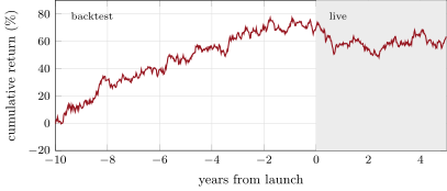
s2_qis.path.The deflated Sharpe ratio (Book 4, chapter 12) asks whether the best of backtests beats what the best of worthless ones would show. Bailey and Lopez de Prado built it to correct for exactly this selection. Applied to each team’s best index, with twenty trials and the team’s own dispersion of backtest Sharpe ratios, it passes 5.9% of them at 95% confidence. Those that pass backtested at 1.13 and live at 0.32 before costs; those that fail, at 0.59 and 0.27. The test is right to be sceptical, but ten years of backtest cannot tell a Sharpe ratio of 0.2 from one of 0.3: the discipline it buys is in the backtests it stops from being sold as excellent, not in picking winners.
Suhonen and co-authors also found that the most complex strategies lost over 30 percentage points more than the simplest. Complexity means more candidates tried, openly or not. In the model, choosing the best of more candidates raises the backtest far more than the live result (Figure 27.2): from 2 to 100 candidates, the best backtest rises from 0.26 to 0.76 and the live Sharpe ratio after costs from 0.07 to 0.24, so the gap between them grows from 0.18 to 0.52. McLean and Pontiff found a related decay in published equity predictors, whose returns were 26% lower out of sample and 58% lower after publication.
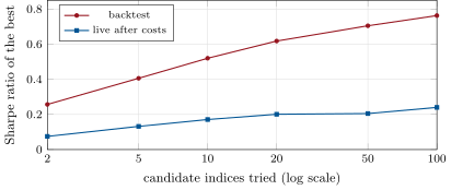
s2_qis.complexity.27.5 Strategy files
Strategy file 27.1 — Risk-premia index swap
Who pays you, and why. Clients who want systematic premia without running them; the bank earns fees and swap margin.
Instruments and venues. Total-return swaps on the bank’s indices; the index’s underlying futures and stocks as the hedge.
Signal. The index rulebook.
Sizing and execution. Hedge by running the index; net its trades with other flows.
Costs. Rebalancing leakage; funding; capital.
How it dies. Live returns far below the backtest; clients leave.
Horizon, capacity, infrastructure. Years; an index calculation agent and a hedging desk.
Backtest honestly. Count every candidate tried; deduct fees and leakage; report the deflated Sharpe ratio.
Sources. Suhonen, Lennkh and Perez (2017); this chapter: backtest 0.51, live after costs 0.16.
Strategy file 27.2 — Volatility-carry index
Who pays you, and why. Buyers of insurance (chapter 1); the index sells it systematically.
Instruments and venues. Index options or variance swaps rolled by rule.
Signal. The rulebook: tenor, strike and size.
Sizing and execution. Fixed notional or volatility-targeted.
Costs. Option spreads; predictable rolls traded ahead.
How it dies. A volatility spike; crowded rolls.
Horizon, capacity, infrastructure. Months; option market access.
Backtest honestly. Include the crashes and the roll costs actually paid.
Sources. Suhonen, Lennkh and Perez (2017) found equity volatility exposures among the more robust live.
Strategy file 27.3 — Multi-asset risk-premia basket
Who pays you, and why. Diversification across carry, momentum, value and volatility premia.
Instruments and venues. Several indices combined in one swap or fund.
Signal. Allocation rules (equal risk).
Sizing and execution. Volatility target at the basket level.
Costs. Each index’s fees and leakage.
How it dies. Premia that fail together; hidden correlation.
Horizon, capacity, infrastructure. Years.
Backtest honestly. Each component’s live record, not its backtest.
Sources. No performance figure verified.
Strategy file 27.4 — Defensive overlay index
Who pays you, and why. Investors paying to cut drawdowns (chapter 7).
Instruments and venues. Trend or put-based indices overlaid on equity holdings.
Signal. The rulebook’s trend or protection rule.
Sizing and execution. Sized to the portfolio it protects.
Costs. The carry cost of protection; fees.
How it dies. Protection that bleeds for years before a crash it misses.
Horizon, capacity, infrastructure. Years.
Backtest honestly. Judge it as insurance: cost against losses avoided, live.
Sources. No performance figure verified.
27.6 Tutorial: written before launch
Goal. Simulate many product teams choosing indices from backtests, charge fees and leakage, compare live with backtest, and test the choice with the deflated Sharpe ratio. End state: the table and two figures.
Teams and launches.
def simulate_teams(cfg: QISConfig | None = None) -> dict:
    cfg = cfg or QISConfig()
    rng = np.random.default_rng(cfg.seed)
    n, k = cfg.teams, cfg.candidates
    true = cfg.sr_mean + cfg.sr_sd * rng.standard_normal((n, k))

    def noise(years):
        common = rng.standard_normal((n, 1))
        own = rng.standard_normal((n, k))
        return (math.sqrt(cfg.corr) * common + math.sqrt(1 - cfg.corr) * own) / math.sqrt(years)

    return {"true": true, "backtest": true + noise(cfg.backtest_years), "live": true + noise(cfg.live_years)}


def launch(sim: dict, cfg: QISConfig | None = None, k: int = 3) -> dict:
    """Launch each team's k best backtests. Live net Sharpe ratio: gross less (fees + leakage) / vol."""
    cfg = cfg or QISConfig()
    order = np.argsort(-sim["backtest"], axis=1)[:, :k]
    pick = lambda a: np.take_along_axis(a, order, axis=1)  # noqa: E731
    bt, live, true = pick(sim["backtest"]), pick(sim["live"]), pick(sim["true"])
    net = live - (cfg.fee + cfg.leakage) / cfg.vol
    return {"backtest": bt, "true": true, "live": live, "net": net,
            "decay_median": float(np.median(1 - net / bt)), "gap": float((bt - net).mean())}
Listing 27.1. Candidates with correlated estimation errors; the best k launched and costed. code/firm/qis/firm_qis.py The deflated verdict.
def deflated(sim: dict, cfg: QISConfig | None = None, threshold: float = 0.95) -> dict:
    """Deflated Sharpe probability of each team's best backtest, with the number of candidates as trials and the
    cross-sectional variance of the team's backtest Sharpe ratios; live results of those that pass and fail."""
    cfg = cfg or QISConfig()
    n_obs = int(cfg.backtest_years * YEAR)
    best = sim["backtest"].argmax(axis=1)
    rows = np.arange(len(best))
    sr_bt = sim["backtest"][rows, best]
    live = sim["live"][rows, best]
    p = np.empty(len(best))
    for i in rows:
        var = sim["backtest"][i].var(ddof=1) / YEAR                       # per-period Sharpe ratio variance
        sr0 = expected_max_sr(cfg.candidates, var)
        p[i] = deflated_sharpe(sr_bt[i] / math.sqrt(YEAR), n_obs, sr0=sr0)
    ok = p > threshold
    return {"prob": p, "pass": float(ok.mean()), "live_pass": float(live[ok].mean()) if ok.any() else float("nan"),
            "live_fail": float(live[~ok].mean()), "bt_pass": float(sr_bt[ok].mean()) if ok.any() else float("nan"),
            "bt_fail": float(sr_bt[~ok].mean())}
Listing 27.2. Each team’s best against the expected best of worthless candidates. code/firm/qis/firm_qis.py - Run
launched(),verdicts(),complexity(),path()andfig_qis.py.
What to change next. Let teams hide failed candidates (count only the survivors) and see the deflated test fooled; add a fee that depends on the backtest; let clients leave after two bad live years.
27.7 Build: quantitative investment strategies
Purpose. Index selection by backtest, fees and leakage, live against backtest, and the deflated Sharpe ratio’s verdict.
Interface. QISConfig(…), simulate_teams(cfg), launch(sim, cfg, k), deflated(sim, cfg), example_path(cfg, team).
Rules. Estimated Sharpe ratios are the truth plus sampling error of ; fees and leakage only live; Book 4’s deflated Sharpe ratio.
Acceptance tests. code/firm/qis/tests/: the sampling error’s size; selection inflates the backtest, not the truth; probabilities in range and the example path’s Sharpe ratio.
Stretch. Non-normal returns; candidates of different complexity; hidden trials.
Sources and further reading
- A. Suhonen, M. Lennkh and F. Perez, “Quantifying backtest overfitting in alternative beta strategies”, Journal of Portfolio Management 43(2), 2017.
- D. H. Bailey and M. Lopez de Prado, “The deflated Sharpe ratio: correcting for selection bias, backtest overfitting, and non-normality”, Journal of Portfolio Management 40(5), 2014.
- R. D. McLean and J. Pontiff, “Does academic research destroy stock return predictability?”, Journal of Finance 71(1), 2016.
27.8 Exercises
Exercise 27.1 ★
An index targets 10% volatility and costs 0.7% a year in fees and leakage. How much Sharpe ratio do the costs take?
Solution
Solution of Exercise 27.1.
of Sharpe ratio.
Exercise 27.2 ★
A backtest over ten years shows a Sharpe ratio of 0.5. What is its standard error, for normal returns?
Solution
Solution of Exercise 27.2.
: a backtest Sharpe ratio of 0.5 is only about 1.6 standard errors from zero before any selection.
Exercise 27.3 ★
Backtest 0.51, live after costs 0.16. What is the decay?
Solution
Solution of Exercise 27.3.
on the means; the median of each index’s own decay is 72.2%, because the ratio is skewed by indices with small backtests.
Exercise 27.4 ★★
Why is the live Sharpe ratio close to the true one while the backtest is far above it?
Solution
Solution of Exercise 27.4.
Live returns were not used to choose the index, so their error averages to zero; the backtest was chosen for being the highest of twenty, so it carries the largest positive errors. Selection biases the statistic it selects on, not the future.
Exercise 27.5 ★★
Why would more complex strategies decay more?
Solution
Solution of Exercise 27.5.
Each rule, filter and parameter added is another set of trials, and the complex strategy’s backtest is the best of more of them; its errors are larger and more of its backtest is noise. Complexity may also fit features of one period that do not recur.
Exercise 27.6 ★★
Why does a published rebalancing schedule cost the index?
Solution
Solution of Exercise 27.6.
Anyone who knows when the index rebalances and roughly what it will trade can buy before it buys and sell before it sells; the index then trades at worse prices than a backtest at historical closes assumes.
Exercise 27.7 ★★★
Coding. Run complexity(). How do the best backtest and the live result change from 2 to 100 candidates, and why does the median decay hardly move?
Solution
Solution of Exercise 27.7.
The best backtest rises from 0.26 with 2 candidates to 0.76 with 100; the live result after costs from 0.07 to 0.24; the gap from 0.18 to 0.52. The median decay stays between 68% and 76% because more candidates also find better strategies: the live result rises too, if much less than the backtest. The gap in Sharpe ratio, not the percentage, is what complexity inflates here.
Exercise 27.8 ★★★
Find the flaw. “The index passed the deflated Sharpe test, so its live Sharpe ratio will be close to its backtest.”
Solution
Solution of Exercise 27.8.
Passing says the best backtest is unlikely to be pure luck, not that it is accurate: those that passed backtested at 1.13 and lived at 0.32 before costs. The selection bias remains in the backtest, and fees and leakage come on top.
27.9 Problem: Written Before Launch
Problem 27.1
Weekend problem — quantitative investment strategies
The chapter’s synthetic product teams and the public record.
Part I — The product.
- Define a quantitative investment strategy and a strategy wrapper.
- How does the bank earn from a QIS?
- Describe the synthetic teams and candidates.
- What is calibrated, and to what?
Part II — Costs.
- What do fees and leakage cost in Sharpe ratio?
- Why are they absent from the backtest?
- How does the bank hedge an index swap?
- What does predictability cost the index?
Part III — Live against backtest.
- Define index backtest decay.
- Give the table of backtest, true and live Sharpe ratios.
- What share of launched indices lose live?
- What does the deflated Sharpe ratio say?
Part IV — The verdict.
- State the named result: the gap between the selected indices’ backtest and live Sharpe ratios.
- What did Suhonen, Lennkh and Perez find?
- What does complexity do in the model?
- What did McLean and Pontiff find?
- How should a client read a QIS backtest?
- Which strategy file did Suhonen and co-authors find most robust?
- How does this chapter relate to Book 7’s chapter on overfitting?
- In one sentence: what does a QIS desk sell?
Solution
Solution of Problem 27.1.
- A bank’s rules-based strategy published as an index and accessed through swaps, notes or funds; the wrapper is the form through which a client holds it.
- Fees, the margin on swaps and notes, and netting the index’s hedges with its other flows.
- 2 000 teams, 20 candidates each with true Sharpe ratios around 0.10 (sd 0.15) and errors correlated at 0.5, ten-year backtests, the best three launched and lived for five years at 10% volatility.
- The distribution of true Sharpe ratios, so the median decay is near the 73% reported for bank-built strategies.
- 0.07 of Sharpe ratio for 0.7% a year at 10% volatility.
- Nobody paid them before the index existed, and a backtest trades at historical prices nobody front-ran.
- By running the index’s positions against the swap.
- Others trade ahead of the published rebalancing; the index buys higher and sells lower.
- The fall from the backtest Sharpe ratio to the live after-cost Sharpe ratio across launched indices.
- Best three: backtest 0.51, true 0.22, live 0.23 before costs and 0.16 after; median decay 72.2%. Best one: 0.62, 0.26, 0.27, 0.20, 69.4%.
- 36.6% have a negative live Sharpe ratio after costs.
- It passes 5.9% of teams’ best indices; those backtested at 1.13 and lived at 0.32, the others at 0.59 and 0.27 before costs.
- The launched indices backtest at a Sharpe ratio of 0.51 and live at 0.16 after costs: a gap of 0.35 and a median decay of 72%.
- A median 73% fall in Sharpe ratio from backtest to live across 215 bank strategies, over 30 points more for the most complex.
- More candidates raise the best backtest from 0.26 to 0.76 and the live result from 0.07 to 0.24: the gap grows from 0.18 to 0.52.
- Published predictors’ returns were 26% lower out of sample and 58% lower after publication.
- As the best of an unknown number of trials, before fees: ask how many were tried, deflate, deduct costs and look for live years.
- The volatility-carry index: equity volatility exposures were among the more robust live.
- This chapter is Book 7’s overfitting, measured on products that were sold.
- Access to a strategy, packaged, costed and hedged, sold on a backtest.
27.10 Interview questions
Interview question 27.1 ★ trader
What is a QIS index, and how does a bank hedge a swap on one?
Solution
Solution of Interview question 27.1.
A rules-based strategy published as an index by a bank, with a rulebook and a calculation agent. The bank that pays the index’s return on a swap hedges by holding the index’s positions, rebalancing them as the rules say.
Interview question 27.2 ★★ researcher
A product team shows you a ten-year backtest with a Sharpe ratio of 1. What do you ask?
Solution
Solution of Interview question 27.2.
How many variants were tried and how the rules were chosen; whether costs, fees and realistic execution are included; what the deflated Sharpe ratio is; how it did in sub-periods and out of sample; and whether any live record exists.
Interview question 27.3 ★★ trader
Other traders front-run your index’s monthly rebalance. What can you change in the rulebook?
Solution
Solution of Interview question 27.3.
Spread the rebalance over several days, randomise its timing within a window, trade on fixings less predictable than the close, or net it internally; each must be written into the rulebook before it applies.
Interview question 27.4 ★★ risk
What risks does a bank keep when it sells swaps on its own indices?
Solution
Solution of Interview question 27.4.
Hedging slippage against the index level, gap and jump risk on rebalancing days, counterparty risk on the swaps, model risk in complex indices, reputational risk from poor live performance, and conflicts between the index sponsor and its trading desk.
Interview question 27.5 ★★ developer
What must an index calculation agent’s system guarantee?
Solution
Solution of Interview question 27.5.
That the index level follows the rulebook exactly, from auditable input prices; that rebalances and corrections are published as the rules say; that historical levels are never silently restated; and that the calculation is independent of the trading desk.
Interview question 27.6 ★★★ researcher
Candidates’ estimated Sharpe ratios are the truth plus independent noise of standard deviation , and the truths are equal. Show that the expected backtest of the best of exceeds its live expectation by about for large .
Solution
Solution of Interview question 27.6.
The best of independent normal errors has expectation about for large (the extreme-value approximation); the live estimate of the chosen candidate has expectation equal to its truth, the same for all. The backtest therefore exceeds the live expectation by about : 0.77 for and , before the slower-converging correction.