Strategies II: Volatility, Relative Value, Macro and the Bank Desks · Strategies
3Skew and Term-Structure Relative Value
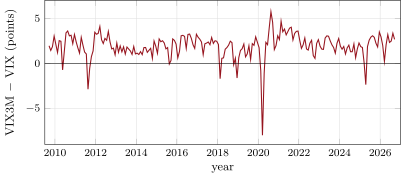
From September 2009 to September 2026 Cboe’s three-month volatility index stood on average 1.93 points above its one-month VIX. On 7.6% of days the order was reversed, and on 12 March 2020 the one-month index stood 18.23 points above the three-month. Two options on the same index, one a month out and one three months out, can disagree about the same future. Relative-value volatility traders bet on the disagreement, or on the shape of the smile, rather than on the level. This chapter builds a synthetic surface whose skew and slope carry planted mispricings that fade, and trades them with vega-neutral, delta-hedged options. The mispricings are real: the parts of the P&L that come from them have Sharpe ratios of 1.0 and 1.5. The trades earn 0.75 and 0.64, and most of what they earn comes from something else. The build is firm.volrv.
3.1 Trading the smile
An index’s implied volatility is higher for low strikes than for high ones: the skew (Book 1, chapter 25). Cboe publishes a measure of it. The SKEW index is , where is the price of S&P 500 skewness computed from a portfolio of options; it rises as the risk-neutral distribution’s left tail grows. From January 1990 to September 2026 it averaged 123.2, with 5% and 95% quantiles of 110.0 and 147.3. Its low was 101.23 on 19 March 1991 and its high 183.12 on 18 February 2025. Cboe’s white paper noted the low correlation between variations in SKEW and VIX. On the history since 1990, daily changes in the two correlate at , and their levels at .
Bakshi, Kapadia and Madan compared the index with its members, using options on the S&P 100 and 30 of its stocks. Individual stocks’ risk-neutral distributions were far less negatively skewed than the index’s. They traced skewness to risk aversion and decomposed each stock’s into a systematic and an idiosyncratic part.
Definition 3.1 (Skew trade)
A skew trade buys options at one strike and sells options at another on the same underlying and expiry, sized so that the position has no net vega and is delta-hedged, in order to profit from a change in the difference between their implied volatilities rather than from the level.
The usual vehicle is the risk reversal (Book 2, chapter 19): long an out-of-the-money call, short an out-of-the-money put, or the reverse. A trader who thinks the put wing is too dear sells the put and buys the call. The trade has a second exposure hidden in it. A surface moves with spot as well as with time: under a sticky-strike rule (Book 5, chapter 7) each strike keeps its vol as spot moves, and under a sticky-delta rule the smile moves with spot. When the index falls, the short put comes nearer the money and its vega grows. The position that had no vega now has some, and it is short.
The synthetic surface
firm.volrv puts a daily surface on the synthetic index of chapter 1. The fair one-month and three-month at-the-money vols come from the variance dynamics, premium included. The fair skew coefficient, the slope of the smile per unit of standardised moneyness , is at the average level. It steepens as the level rises: 0.4 of a unit of skew for each unit of one-month vol. On top of the fair surface the market adds two planted noises: one on the skew coefficient (standard deviation 0.06) and one on the three-month vol (1.5 vol points). Each is an autoregression with a daily persistence of 0.98, a half-life of 34 days. They stand for demand that pushes one part of the surface and then fades. The smile is .
A trader does not see the noises. features extracts what can be seen: the level (the one-month vol), the slope (three-month minus one-month) and the skew. It then regresses slope and skew on the level, using only data up to each day, and keeps the residuals. The raw skew correlates with the level at and the raw slope at . The full-sample fits give for the skew’s level beta (the planted value is ) and for the slope’s. The residuals recover the planted noises well: they correlate with them at 0.97 for the skew and 0.92 for the slope.
3.2 Trading the term structure
Definition 3.2 (Term-structure trade)
A term-structure trade buys volatility at one maturity and sells it at another on the same underlying, sized so that the position has no net vega and is delta-hedged, in order to profit from a change in the slope of the term structure rather than from the level.
The calendar spread is the standard form: long three-month, short one-month at-the-money options with equal vegas. Its shape follows from how vol mean-reverts. When vol is high, the market expects it to fall, so near-dated vol stands above far-dated vol and the term structure inverts. When vol is low, the order reverses. A slope is therefore, in large part, a level in disguise. On the real indices (Figure 3.1) the slope VIX3M minus VIX correlates with VIX at . It averaged points through March 2020. It is also quick to revert: its daily persistence is 0.90, a half-life of 6.5 trading days.
s2_fetch_term.Johnson studied what the slope says. The shape of the VIX term structure carries information about the price of variance risk, not about expected changes in VIX, which rejects the expectations hypothesis. Its second principal component, a slope, predicts the excess returns of synthetic S&P 500 variance swaps, VIX futures and S&P 500 straddles at all maturities. A trader can read this two ways. It is a timing signal for the level trades of chapter 1: sell variance when the slope says the premium is high. It is also a warning for a calendar spread, which trades the slope itself.
3.3 Across related underlyings
Definition 3.3 (Cross-underlying volatility spread)
A cross-underlying volatility spread buys implied volatility on one underlying and sells it on a related one, such as two indices, an index and an exchange-traded fund on it, or an index and its members, betting that the ratio or difference of the two vols returns to its usual range.
Cboe publishes volatility indices for the Russell 2000 (RVX) and the Nasdaq-100 (VXN). Since September 2009, RVX has stood on average 5.2 points above VIX, with a standard deviation of 2.3 points and a half-life of 15.7 trading days. VXN has stood 3.0 points above, with a standard deviation of 2.3 and a half-life of 15.3 days. The spreads revert more slowly than the VIX slope, and nothing in them is the level of one market in disguise. That makes them the cleanest relative-value signal of this chapter. It also brings the least familiar risk. The two underlyings can part company for a reason (a sector’s crash, a change in an index’s membership), and the spread then does not come back.
Nobody trades the volatility indices themselves: the trade is in options on each underlying. It carries each underlying’s delta hedge, each option market’s spread, and the chance that one surface is quoted less often than the other. Bakshi, Kapadia and Madan’s result is the basis of the most common cross-underlying trade, index skew against single-stock skew. Its risk is the correlation of chapter 2.
3.4 The books and their attribution
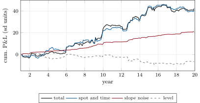
Each month the book strikes a unit trade scaled by minus the signal, an expanding z-score clipped at 2: it sells what is rich. The trade is a risk reversal one standardised unit either side of the money, or a one-month against three-month calendar. Each leg is sized so that a one-percent rise in its vol is worth one unit (0.18 vol points at a vol of 18). Every leg is delta-hedged daily and held to the month’s end. Opening a leg costs one percent of its vol, the chapter’s own assumption rather than a sourced spread. The P&L is attributed each day by repricing in order (Listing 3.1): spot and time (delta, gamma, theta, on the day’s surface), then the level (the fair surface moving to the next day’s), then the skew noise, then the slope noise. The order matters: the level is moved first, and the skew and slope buckets hold only the planted noises. Four books run over 227 months after a year’s warm-up: each trade, signalled by the raw feature or by its residual on the level.
| share of P&L (%) | |||||||
| 227 months | Sharpe | skewness | worst (sd) | spot, time | level | skew or slope | cost |
| skew, raw | 1.13 | 1.91 | 94 | 5 | 9 | ||
| skew, residual | 0.75 | 1.48 | 73 | 24 | 16 | ||
| calendar, raw | 0.07 | 4.74 | 160 | 155 | |||
| calendar, residual | 0.64 | 1.43 | 97 | 51 | |||
The planted effects are there. Taken alone, the skew bucket of the residual skew book has a Sharpe ratio of 1.01 and the slope bucket of the residual calendar 1.51. The raw books catch less of them: 0.95 for the raw skew book’s skew bucket and 0.84 for the raw calendar’s slope bucket. But these buckets are small next to the rest. The planted skew noise explains 16% of the residual skew book’s P&L. The skew book signalled on the raw feature has the highest Sharpe ratio of the four, and only 9% of its P&L comes from the skew moving back. The rest is spot and time. The raw skew is steep when vol is high, so this book sells the put wing when vol is high. What it collects is chapter 1’s premium, with a risk reversal’s paperwork.
The raw calendar is the other case. Its slope signal is 83% level, so its level bucket (160% of the P&L) and its slope bucket (155%) are both large, and costs take the difference. The residual calendar keeps the slope bucket and sheds most of the level. Half its P&L is the planted effect. The other half is spot and time, and part of that is the mispricing too: an option bought cheap earns more from gamma than it pays in theta while it is held. Across months the spot-and-time bucket correlates with the size of the mispricing held at 0.25 for the skew book and 0.14 for the calendar. The rest is gamma noise, and it dominates the month-to-month variance (Figure 3.2).
s2_volrv.books.One seed can flatter a book. Over eight seeds of the market and the surface, the mean Sharpe ratios are 0.90 for the raw skew book (range 0.47 to 1.26), 0.39 for the residual skew book (0.12 to 0.75), for the raw calendar ( to 0.29) and 0.38 for the residual calendar ( to 0.75). The chapter’s seed is on the lucky side for both residual books.
3.5 Risk: what a relative-value vol book is really short
A book with no net vega and no net delta at inception is not a book without risk. Held every month without a signal, one unit of each trade shows what it carries. Long the call wing and short the put earns 12.0 units a month from spot and time and loses 15.9 to the level: a month in all. Its short put gains vega as the index falls, when vol rises. Long the calendar earns 9.6 units a month from spot and time, since the short one-month leg collects the variance premium through theta, and loses 3.2 to the level: 4.7 a month in all.
The worst month of both skew books began on day 1 470 (year 5.8). Both books were at their limit: two units long the call wing and short the put. The crash came nine days after the month ended. Inside the month the index rose 4.5% while the one-month vol fell from 15.2% to 9.7%. The long call rose to its strike and its vega grew just as the vol it was long collapsed. The month cost 289 units: 119 from spot and time (the call’s theta in a calm rally) and 157 from the level, 4.5 of the book’s monthly standard deviations. The residual signal had no way to see it coming: the skew noise was steep that month and said to sell the put wing. A relative-value vol book is short whatever its legs do not match. For a risk reversal that is a joint move of spot and vol in either direction: a crash when it is short the put wing, a calm rally with falling vol when it is long the call. For a calendar it is gamma in the near month, which the three-month leg does not cover.
Three rules follow. Attribute before believing a Sharpe ratio: a skew trade whose skew bucket is a tenth of its P&L is a different trade. Signal on residuals to the level, or the book is a level trade with extra costs. Stress each book on joint moves of spot, vol and skew in both directions, not on one of them at a time.
3.6 Strategy files
Strategy file 3.1 — Skew flattener
Who pays you, and why. Hedgers who bid index puts beyond what the surface’s other points justify; the payment is the part of the put wing’s richness that fades.
Instruments and venues. Listed index options, out-of-the-money puts and calls of one expiry.
Signal. The skew’s residual after its dependence on the level, against its history.
Sizing and execution. Vega-neutral risk reversals, delta-hedged daily; sized by the crash-month loss, not by the Sharpe ratio.
Costs. Two option spreads a roll and the hedging; the put wing is the less liquid.
How it dies. A crash while short the put wing; a skew that steepens with the level and never comes back.
Horizon, capacity, infrastructure. Weeks to months; a daily surface fit and a hedging engine.
Backtest honestly. Attribute the P&L; test the raw and residual signals; include crash months.
Sources. Bakshi, Kapadia and Madan (2003) on index skew; this chapter: 0.75 on one seed, 0.39 on average over eight, with 16% of the P&L from the skew.
Strategy file 3.2 — Calendar volatility spread
Who pays you, and why. Demand concentrated at one maturity (hedgers in the near month, structured-product issuers further out) that fades.
Instruments and venues. Listed index options at two expiries; variance swaps or VIX futures at two tenors.
Signal. The slope’s residual after its dependence on the level.
Sizing and execution. Equal vegas; delta-hedged; near leg rolled monthly.
Costs. Two spreads a roll; the near leg’s hedging.
How it dies. A vol spike, when the short near leg’s gamma loses; a slope signal that is really the level.
Horizon, capacity, infrastructure. Weeks to months; a term-structure fit.
Backtest honestly. Signal on residuals; attribute to level and slope; include inversions.
Sources. Johnson (2017) on the VIX slope and variance risk premia; this chapter: 0.64 on one seed, 0.38 on average.
Strategy file 3.3 — Index-versus-ETF volatility spread
Who pays you, and why. Flows that hit one of two option markets on nearly the same underlying, such as index options against options on an exchange-traded fund that tracks the index.
Instruments and venues. Index options against the fund’s options; the fund’s tracking and dividends set the fair spread.
Signal. The implied-vol difference against the tracking-adjusted fair difference.
Sizing and execution. Vega-neutral, delta-hedged in each underlying.
Costs. Two option markets’ spreads; different settlement and exercise styles.
How it dies. Differences that are fair (exercise style, settlement, dividends, taxes) mistaken for mispricing.
Horizon, capacity, infrastructure. Days to weeks; both surfaces live.
Backtest honestly. Model settlement and exercise differences before calling a gap a signal.
Sources. No performance figure verified.
Strategy file 3.4 — Cross-market volatility spread
Who pays you, and why. Demand for protection on one market that pushes its vol away from a related market’s.
Instruments and venues. Options or volatility futures on two indices (small caps against large caps, one region against another).
Signal. The vol spread or ratio against its history; Cboe’s RVX and VXN against VIX revert with half-lives of about 15 days.
Sizing and execution. Vega-neutral or beta-weighted legs.
Costs. Two markets’ spreads and hedges.
How it dies. A regime change in one market: the spread moves and stays.
Horizon, capacity, infrastructure. Weeks; two surfaces.
Backtest honestly. Test whether the spread reverts after a shock or trends.
Sources. Cboe’s RVX, VXN and VIX histories (statistics in this chapter); no performance figure verified.
3.7 Tutorial: same future, two prices
Goal. Build the synthetic surface, extract its features, run the four books and attribute their P&L; read the real term structure, SKEW and cross-index spreads. End state: the table and the two figures.
The trade and its attribution.
def trade_pnl(r, s: dict, kind: str, pos, cfg, scfg: SurfaceConfig | None = None) -> dict:
    """Per-period P&L buckets of pos[start] unit trades struck every roll_days and held, delta-hedged daily, for the
    period (kind 'skew' or 'calendar'). Each leg is sized so that a one-percent rise in its vol is worth one unit at
    inception: P&L is in percent of vol, whatever the level."""
    scfg = scfg or SurfaceConfig()
    st = lambda t, a3, sk: (s["atm1"][t], a3, sk)                                   # noqa: E731
    starts = np.arange(0, len(r) - scfg.roll_days - 1, scfg.roll_days)
    out = {k: np.zeros(len(starts)) for k in ("spot_time", "level", "skew", "slope", "cost")}
    for i, t0 in enumerate(starts):
        p = float(pos[t0])
        now0 = st(t0, s["atm3"][t0], s["skew"][t0])
        for tau0, x, right, sign in _legs(kind):
            K = float(np.exp(x * _atm(now0, tau0) * np.sqrt(tau0)))
            q = sign * p / (_value((now0[0] * 1.01, now0[1] * 1.01, now0[2]), 1.0, K, tau0, right, cfg.curv)[0]
                            - _value(now0, 1.0, K, tau0, right, cfg.curv)[0])
            S = 1.0
            for d in range(scfg.roll_days):
                t, tau = t0 + d, tau0 - d / YEAR
                S1 = S * np.exp(r[t + 1])
                now = st(t, s["atm3"][t], s["skew"][t])
                lvl = (s["atm1"][t + 1], s["fair3"][t + 1] + s["e_slope"][t], s["fair_skew"][t + 1] + s["e_skew"][t])
                skw = (lvl[0], lvl[1], s["skew"][t + 1])
                nxt = st(t + 1, s["atm3"][t + 1], s["skew"][t + 1])
                v0, delta = _value(now, S, K, tau, right, cfg.curv)
                v1, v2, v3, v4 = (_value(z, S1, K, tau - 1 / YEAR, right, cfg.curv)[0] for z in (now, lvl, skw, nxt))
                out["spot_time"][i] += q * (v1 - v0 - delta * (S1 - S))
                out["level"][i] += q * (v2 - v1)
                out["skew"][i] += q * (v3 - v2)
                out["slope"][i] += q * (v4 - v3)
                S = S1
        out["cost"][i] = -100 * scfg.half_spread * 2 * abs(p)                     # both legs opened each period
    out["total"] = sum(out[k] for k in ("spot_time", "level", "skew", "slope", "cost"))
    out["start"] = starts
    return out
Listing 3.1. A unit trade struck monthly, delta-hedged daily, attributed by sequential repricing. code/firm/volrv/firm_volrv.py Signals and books.
def zscore(x, warmup: int = 252, cap: float = 2.0):
    """Expanding z-score using data up to each day only, clipped at +-cap; zero during the warm-up."""
    x = np.asarray(x, float)
    n = np.arange(1, len(x) + 1)
    m = np.cumsum(x) / n
    sd = np.sqrt(np.maximum(np.cumsum(x * x) / n - m * m, 1e-18))
    out = np.zeros(len(x))
    out[warmup:] = ((x - m) / sd)[warmup:]
    return np.clip(out, -cap, cap)


@functools.lru_cache(maxsize=16)
def market(seed: int = 0, noise: float = 1.0):
    """The synthetic index and surface; noise scales both planted noises (0 switches them off)."""
    cfg, base = VolConfig(seed=91 + seed), SurfaceConfig(seed=93 + seed)
    sim = simulate_vol(cfg)
    scfg = SurfaceConfig(seed=93 + seed, skew_sd=noise * base.skew_sd, slope_sd=noise * base.slope_sd)
    s = surface_path(sim["r"], sim["v"], cfg, scfg)
    return cfg, sim, s, features(s)


@functools.lru_cache(maxsize=16)
def books(seed: int = 0, noise: float = 1.0):
    """Each book's monthly P&L buckets: sell what is rich, so hold minus the z-scored feature."""
    cfg, sim, s, f = market(seed, noise)
    out = {}
    for name, kind, feat in BOOKS:
        b = trade_pnl(sim["r"], s, kind, -zscore(f[feat]), cfg)
        out[name] = {k: v[WARMUP:] for k, v in b.items()}
    return out
Listing 3.2. Expanding z-scores and the four books. code/strategies-2/03-skew-and-term-structure-relative-value/python/s2_volrv.py - Run
s2_fetch_term.pyonce, thentable(),bucket_sr(),seeds(),static()andfig_volrv.py.
What to change next. Hedge the risk reversal’s crash exposure with a small long put further out and measure what it costs; switch the surface’s rule to sticky delta and compare the attributions; add a third maturity and trade the curvature of the term structure.
3.8 Build: volatility relative value
Purpose. A daily surface with planted skew and slope mispricings; surface features and their residuals on the level; vega-neutral risk reversals and calendars with P&L attribution.
Interface. SurfaceConfig(…), surface_path(r, v, cfg, scfg), features(s, warmup), trade_pnl(r, s, kind, pos, cfg, scfg), attribution(b).
Rules. Residuals from expanding regressions only; legs sized by relative vega at inception; attribution in a fixed order (spot and time, level, skew, slope) so that the buckets add up to the total.
Acceptance tests. code/firm/volrv/tests/: a linear level effect removed exactly; a still surface gives no level, skew or slope P&L and buckets that add up; a risk reversal gains when the skew flattens and loses when reversed.
Stretch. Sticky-delta dynamics; curvature trades; two underlyings.
Sources and further reading
- G. Bakshi, N. Kapadia and D. Madan, “Stock return characteristics, skew laws, and the differential pricing of individual equity options”, Review of Financial Studies 16(1), 2003.
- T. L. Johnson, “Risk premia and the VIX term structure”, Journal of Financial and Quantitative Analysis 52(6), 2017.
- Cboe, SKEW Index white paper, 2011.
- Cboe Global Markets, daily histories of VIX, VIX3M, SKEW, RVX and VXN.
3.9 Exercises
Exercise 3.1 ★
The price of S&P 500 skewness is . What is the SKEW index?
Solution
Solution of Exercise 3.1.
.
Exercise 3.2 ★
A leg is sized so that a one-percent rise in its vol is worth one unit. Its vol is 20% and falls to 19.6%. What does a short position in the leg make?
Solution
Solution of Exercise 3.2.
The vol falls by of itself, so the short position makes 2 units.
Exercise 3.3 ★
An autoregression has daily persistence 0.98. What is its half-life in trading days?
Solution
Solution of Exercise 3.3.
trading days.
Exercise 3.4 ★★
Why is a calendar spread signalled on the raw slope largely a trade on the level of vol?
Solution
Solution of Exercise 3.4.
Vol mean-reverts, so the fair term structure inverts when vol is high and slopes up when it is low: the raw slope correlates with the level at on the synthetic surface and on the real VIX curve. Buying the calendar when the slope is low means buying it when vol is high, a bet that vol falls. The residual on the level removes most of that.
Exercise 3.5 ★★
Johnson found that the VIX slope predicts variance-swap, VIX-future and straddle returns. How would you use that finding in a level trade, and what does it warn a calendar trader about?
Solution
Solution of Exercise 3.5.
As a timing signal for the short-variance trades of chapter 1: sell variance when the slope says the variance premium is high. For a calendar trader the finding says the slope is mostly the price of variance risk, not a forecast of vol, so a calendar signalled on the slope is exposed to the variance premium, the level trade it was meant to avoid.
Exercise 3.6 ★★
Individual stocks’ risk-neutral distributions are less negatively skewed than the index’s. Design a trade on that difference and name its main risk.
Solution
Solution of Exercise 3.6.
Sell the index’s put skew and buy the members’ put skew (a risk reversal on the index against risk reversals on the members), vega-neutral and delta-hedged. Its main risk is correlation: in a crash every member falls with the index and the index skew’s richness is justified, which is chapter 2’s dispersion risk in skew form.
Exercise 3.7 ★★★
Coding. Run table(0, 0.0), which switches off both planted noises. What happens to each book, and what does it tell you about the raw skew book?
Solution
Solution of Exercise 3.7.
The raw skew book still earns a Sharpe ratio of 1.08 (worst month standard deviations): it never needed the planted effect, because it is selling the put wing when vol is high. The residual skew book loses (, a worst month of standard deviations), since its signal is now only the regression’s error. Both calendars lose ( raw, residual) to costs and gamma.
Exercise 3.8 ★★★
Find the flaw. “Our skew book has a Sharpe ratio of 1.13 and the skew mean-reverts, so we are being paid for skew mean reversion.”
Solution
Solution of Exercise 3.8.
The attribution says otherwise. Only 9% of that book’s P&L comes from the skew moving back, 94% from spot and time; the raw skew is steep when vol is high, so the book is selling the put wing when vol is high. With the planted noise switched off it still earns 1.08. The Sharpe ratio is real, but it pays for the variance premium and the crash risk that comes with it, not for skew mean reversion.
3.10 Problem: Same Future, Two Prices
Problem 3.1
Weekend problem — relative value on a surface
The chapter’s synthetic surface, Cboe’s indices and the public record.
Part I — The surface.
- Define a skew trade and a term-structure trade.
- How is Cboe’s SKEW index defined, and what were its statistics?
- What did Bakshi, Kapadia and Madan find about index and stock skews?
- How does the synthetic surface’s fair skew depend on the level, and what are its planted noises?
Part II — The real term structure.
- Give the VIX slope’s average, how often it was inverted, and its extreme.
- Why does the slope correlate with the level?
- What did Johnson find?
- Give the RVX and VXN spreads to VIX and their half-lives.
Part III — The books.
- How are the features and their residuals extracted?
- How is each leg sized, and in what units is the P&L?
- How is the P&L attributed, and why does the order matter?
- Give the four books’ Sharpe ratios and their attributions.
Part IV — The verdict.
- State the named result: the skew and calendar trades’ Sharpe ratios and the share of their P&L that is really something else.
- What do the planted effects earn alone?
- What did the eight seeds show?
- What does each trade carry when held without a signal?
- What happened in the worst month of the skew books?
- What happens when the planted noises are switched off?
- How would you backtest a skew book honestly?
- In one sentence: what is a relative-value vol book short?
Solution
Solution of Problem 3.1.
- A skew trade: long and short options at two strikes of one expiry, vega-neutral and delta-hedged, on the difference in their vols. A term-structure trade: the same across two maturities.
- , with the price of S&P 500 skewness; 123.2 on average since 1990, 110.0 to 147.3 for the middle 90%, 101.23 at the low (19 March 1991) and 183.12 at the high (18 February 2025).
- Individual stocks’ risk-neutral distributions are far less negatively skewed than the index’s.
- The fair skew is at the average level and moves by per unit of one-month vol; the noises are an AR(1) on the skew (sd 0.06) and on the three-month vol (1.5 vol points), with a half-life of 34 days.
- 1.93 points on average; inverted on 7.6% of days; on 12 March 2020.
- Vol mean-reverts, so high vol inverts the curve; the correlation is .
- The slope carries the price of variance risk and predicts variance-swap, VIX-future and straddle returns.
- RVX 5.2 points above VIX (sd 2.3, half-life 15.7 days); VXN 3.0 above (sd 2.3, half-life 15.3).
- Level, slope and skew from the surface; slope and skew regressed on the level with expanding windows, keeping the residuals.
- One unit per one-percent rise in the leg’s vol at inception; P&L in percent of vol.
- Repricing in order: spot and time, then level, then skew noise, then slope noise; the buckets add up, and moving the level first puts the fair skew and slope changes in the level bucket.
- 1.13, 0.75, 0.07 and 0.64; spot and time 94, 73, and 97%; level 5, 24, 160 and %; skew or slope 9, 16, 155 and 51%.
- Named result. The skew and calendar trades signalled on residuals earn Sharpe ratios of 0.75 and 0.64 on this seed (0.39 and 0.38 on average over eight). Only 16% and 51% of their P&L comes from the planted skew and slope; the raw skew book earns 1.13 with 9%, and the raw calendar’s P&L is 160% level.
- Sharpe ratios of 1.01 (skew bucket) and 1.51 (slope bucket).
- Means of 0.90, 0.39, and 0.38; this seed is on the lucky side for the residual books.
- The risk reversal: 12.0 units a month from spot and time, from the level, in all. The calendar: 9.6, , 4.7.
- Long two units of call wing into a 4.5% rally with the one-month vol falling from 15.2% to 9.7%: units, 4.5 standard deviations.
- The raw skew book still earns 1.08; the residual books and calendars lose.
- Attribute the P&L, compare raw and residual signals, include joint moves of spot and vol, charge option costs, report several seeds.
- Whatever its legs do not match: the joint moves of spot and vol, and near-month gamma.
3.11 Interview questions
Interview question 3.1 ★ trader
What is a risk reversal, and what does its price tell you?
Solution
Solution of Interview question 3.1.
Long an out-of-the-money call and short an out-of-the-money put (or the reverse) at equal deltas or vegas. Its price, quoted as the call’s vol minus the put’s, measures the skew: a large negative value says the put wing is dear.
Interview question 3.2 ★★ trader
You are long a vega-neutral calendar. The market sells off sharply. What happens to your P&L?
Solution
Solution of Interview question 3.2.
Vol rises and the curve inverts: the short one-month leg’s vol rises more than the long three-month’s, so the level move loses; the short near leg has more gamma than the long far leg, so the large moves lose too. Both hurt.
Interview question 3.3 ★★ researcher
How would you tell whether a skew signal is a level signal in disguise?
Solution
Solution of Interview question 3.3.
Regress the skew on the level and check the correlation; trade the residual as well as the raw signal and compare; attribute the P&L into level and skew buckets. If the raw signal’s P&L is mainly spot, time or level, it is a level signal.
Interview question 3.4 ★★ risk
A relative-value vol book reports zero vega and zero delta. What risks remain?
Solution
Solution of Interview question 3.4.
Gamma and theta that do not cancel; vega that appears as spot moves (a short wing coming to the money); the joint move of spot, vol and skew; jumps between hedges; basis between underlyings; the costs of rolling and hedging.
Interview question 3.5 ★★ developer
Design a daily P&L attribution for an options book. What has to be true for the buckets to add up?
Solution
Solution of Interview question 3.5.
Reprice each position in a fixed order of market moves (spot and time, then level, then shape parameters) and record each step’s change; the last state must equal the next day’s full surface, so the buckets add to the total by construction. The surface must be a function of a small set of parameters, with a rule for how it moves with spot.
Interview question 3.6 ★★★ researcher
Under Black–Scholes, show that a delta-hedged option’s P&L over a short interval is approximately , and explain why two legs of equal vega but different implied vols do not have equal gamma.
Solution
Solution of Interview question 3.6.
Over the hedged option’s value changes by , and Black–Scholes gives ; with the P&L is . Vega is and gamma , so gamma per unit of vega is : the leg with the higher implied vol has less gamma per unit of vega.