Strategies II: Volatility, Relative Value, Macro and the Bank Desks · Strategies

22Storage, Transport and Physical Optionality

A trader who leases a gas storage cavern owns a string of calendar spread options; one who holds pipeline capacity owns location spread options. The physical asset is valued as the options it contains, and the trader’s job is to turn them into money with hedges. Secomandi found that most of the value of adapting to price uncertainty can be generated simply by re-optimising, again and again, a plan that ignores the uncertainty. On this chapter’s synthetic lease, locking today’s best plan is worth $716 000. Re-optimising it each month on the new forward curve and re-hedging adds $56 800 on average, and on no path does it earn less. At two cents per unit of forward traded it adds $26 600 and loses to the locked plan on a third of paths. The build is firm.physopt.

22.1 Storage as an option

Definition 22.1 (Storage deal)

A storage deal is a lease of storage capacity (working volume and injection and withdrawal rates, for a period) that the trader monetises by buying the commodity when it is cheap, holding it and selling when it is dear, hedging each planned injection and withdrawal in the forward market.

The lease in firm.physopt holds 10 units of 100 000 MMBtu, injects up to 2 units and withdraws up to 4 a month, and costs 2 cents per MMBtu each way. The forward curve and the price model are Book 6’s (chapter 16): an illustrative Henry Hub-like curve from April ($2.60) to January ($3.50) and a two-factor model with 60% short-end and 20% long-end volatility. The intrinsic plan buys 2 units in each month from April to August and sells 4 in December, 4 in January and 2 in February. Locked with forwards, it is worth $716 000.

Four valuation methods give four numbers:

method	value ($ thousands)
intrinsic: today’s best plan, locked	716
spread options: the plan’s ten injection-withdrawal pairs, each an option	722
least-squares Monte Carlo on spot (Book 6)	760
rolling intrinsic: re-optimised each month, hedges traded	773

The spread-option method pairs each unit injected with a unit withdrawn, first in first out, and values each pair as a calendar spread option on the two forwards struck at the operating costs (Listing 22.2). Here the pairs are deep in the money and add little. Least-squares Monte Carlo acts on spot prices alone and estimates continuation values by regression, which loses a little. Rolling intrinsic uses the whole forward curve each month. Lai, Margot and Secomandi found that practitioners’ heuristics are fast but significantly suboptimal, and that with periodic re-optimisation inside a Monte Carlo simulation they become nearly optimal, with one exception.

22.2 Monetising the options

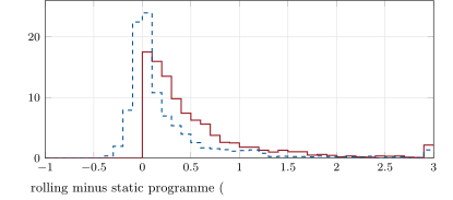
The value is realised through a hedge programme (Listing 22.1). The static programme buys forwards for every planned injection and sells forwards for every planned withdrawal, 20 units in all, and delivers the plan at spot. Whatever the prices do, it earns $716 000: the hedges’ gains and losses exactly offset the spot prices paid and received. The rolling programme re-optimises the plan each month on the simulated forward curve, given the gas already in store, and trades the difference in hedges. A new plan is chosen only if it is worth more on the current curve than the old one, and the hedges lock that gain; so, without trading costs, rolling can never earn less than the static programme on any path.

cost per unit of forward traded	0	0.5 cent	2 cents	2 cents, gated
extra over the static programme ($ thousands)	56.8	49.2	26.6	37.4
paths below the static programme	0%	3.1%	32.6%	0%
extra units of forward traded	15.1	15.1	15.1	9.2

The static programme also pays for its own 20 units of hedges, so the comparison is at equal costs. At two cents per unit the rolling programme still earns more on average, but it loses to the static one on a third of paths, because it re-hedges whenever the new plan is better by any amount (Figure 22.1). The gated version re-hedges only when the gain on the curve exceeds the cost of the trades. It trades 9.2 extra units instead of 15.1, earns $37 400 more than the static programme on average and never less.

Distribution over 2 000 simulated paths of the rolling-intrinsic programme’s P&L less the static programme’s, without trading costs and at 2 cents per unit of forward traded; the end bins collect the tails. Data: s2_physopt.programmes. — **Figure 22.1.** Distribution over 2 000 simulated paths of the rolling-intrinsic programme’s P&L less the static programme’s, without trading costs and at 2 cents per unit of forward traded; the end bins collect the tails. Data: `s2_physopt.programmes`.

22.3 Transport as an option

Definition 22.2 (Transport option)

A transport option is the right, given by pipeline or shipping capacity, to move a commodity from one location to another in a period at a variable cost; it is worth a spread option on the destination price less the origin price, struck at that cost.

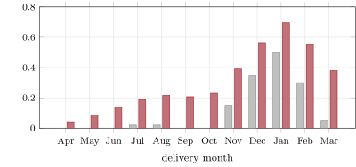
Capacity of 1 unit a month from the hub to a market-area hub, whose forwards stand above the hub’s by 5 cents in spring to 60 cents in January, with a variable cost of 10 cents, is worth $139 000 on today’s forwards: only the winter months pay. As a strip of spread options, with volatilities of 45% and 55% and a correlation of 0.85, it is worth $369 000 (Figure 22.2). Its value depends on how independently the two hubs move: $580 000 at a correlation of 0.5 and $273 000 at 0.95. The holder monetises it like storage: by selling the spread forward in the months it is in the money, and re-optimising as the basis moves.

A year of monthly transport capacity from the hub to a market-area hub: the intrinsic value on today’s forwards and the spread-option value of each month, per MMBtu. Data: s2_physopt.transport_strip. — **Figure 22.2.** A year of monthly transport capacity from the hub to a market-area hub: the intrinsic value on today’s forwards and the spread-option value of each month, per MMBtu. Data: `s2_physopt.transport_strip`.

A cargo of liquefied natural gas committed to Europe at $10.00 per MMBtu that can instead go to Asia at $10.50, for 80 cents more in shipping, has no intrinsic value in switching. The switch is still an option on the Asian price less the European price, struck at 80 cents: with three months to decide, volatilities of 60% and a correlation of 0.8, it is worth 64 cents per MMBtu, and $1.08 at a correlation of 0.5.

22.4 What the asset-backed trader owns

Definition 22.3 (Asset-backed trading)

Asset-backed trading is trading around physical assets that the firm owns or leases (storage, transport capacity, generation, cargoes), valuing them as options and monetising their flexibility with hedges in the forward and options markets.

The asset-backed trader owns three things a financial trader does not. The first is the options themselves, which cannot be bought on an exchange. The second is the obligation to operate them, with the physical constraints that make the options valuable and the plans complicated. The third is information: flows through the asset show supply and demand before prices do. What the trader does not own is certainty that the spreads will be there. From 2007 to 2025, the Henry Hub winter spot price (December to February) was above the preceding summer’s (April to June) in 12 of 19 years. It averaged 7 cents less, with a standard deviation of $2.04. In 2008 the winter was $6.12 below the summer, and in 2022 $3.71. An operator who injected and waited without hedging earned those numbers. The hedge programme exists to replace them with the forward spread at the time of the decision.

22.5 Strategy files

Strategy file 22.1 — Rolling-intrinsic storage

Who pays you, and why. Consumers who pay a winter premium; the forward curve’s seasonal spread pays for holding gas through the summer.

Instruments and venues. A storage lease; monthly gas forwards or futures.

Signal. The best plan on the current forward curve.

Sizing and execution. Hedge the whole plan; re-optimise monthly or on large moves; re-hedge only when the gain exceeds the cost.

Costs. The lease; injection and withdrawal fees; forward bid-ask.

How it dies. Lease costs above the value; flat curves; operational outages.

Horizon, capacity, infrastructure. A storage year; scheduling and nominations.

Backtest honestly. Forward curves as they were; physical constraints enforced; costs on every re-hedge.

Sources. Secomandi (2010); Lai, Margot and Secomandi (2010); this chapter: $56 800 above intrinsic without costs.

Strategy file 22.2 — Spread-option storage hedge

Who pays you, and why. Buyers of calendar spread options who want the flexibility the storage owner has.

Instruments and venues. Calendar spread options on gas futures; over-the-counter spread options.

Signal. The storage’s option value against the options’ market price.

Sizing and execution. Sell the options the facility can deliver: pairs of injection and withdrawal months.

Costs. Option bid-ask.

How it dies. Selling more optionality than the facility’s rates allow.

Horizon, capacity, infrastructure. A season.

Backtest honestly. Exercise constrained by the facility’s rates.

Sources. This chapter: the pairs are worth $722 000 against $716 000 intrinsic.

Strategy file 22.3 — Transport capacity optimisation

Who pays you, and why. Buyers in constrained market areas; the basis pays for the pipe.

Instruments and venues. Pipeline capacity; basis swaps or futures at both hubs.

Signal. The forward basis against the variable cost.

Sizing and execution. Sell the basis forward in months in the money; re-optimise as it moves.

Costs. Capacity charges; fuel; basis bid-ask.

How it dies. New pipelines that close the basis; correlation that rises.

Horizon, capacity, infrastructure. Seasons to years; nominations.

Backtest honestly. Basis at both hubs as it was; capacity outages.

Sources. This chapter: $139 000 intrinsic, $369 000 as options.

Strategy file 22.4 — Cargo diversion

Who pays you, and why. Markets that bid for flexible supply when tight.

Instruments and venues. LNG cargoes with destination flexibility; regional gas futures; freight.

Signal. Netbacks by destination: price less shipping and regasification.

Sizing and execution. Hedge the committed destination; hold the switch as an option.

Costs. Shipping, boil-off, canal and port charges.

How it dies. Contract restrictions; freight spikes; converging regional prices.

Horizon, capacity, infrastructure. Weeks to months; shipping and scheduling.

Backtest honestly. Freight and netbacks at the decision date.

Sources. This chapter: 64 cents per MMBtu at a correlation of 0.8.

22.6 Tutorial: the asset as options

Goal. Value a storage lease four ways, run its static and rolling hedge programmes path by path with trading costs, and value transport capacity and a cargo switch as spread options. End state: the two tables and two figures.

The hedge programme.

def hedge_programme(fac: Facility, model: TwoFactor, F0: list[float], T: list[float], paths: int = 2000,
                    seed: int = 5, cost: float = 0.0, roll: bool = True, gate: bool = False) -> dict:
    """Lock the intrinsic plan with forwards (long what will be injected, short what will be withdrawn); with `roll`,
    re-optimise at each month on the simulated curve and trade the change in hedges at `cost` per unit; with `gate`,
    only where the new plan's value on the curve beats the old plan's by more than that cost. Returns the intrinsic
    value and, per path, the realised P&L and the units of forward traded."""
    chi, xi = model.simulate(T, paths, seed)
    n, rows = len(T), chi.shape[0]
    first = plans(fac, np.array([F0], float), np.array([fac.start]))[0]
    value0 = float(sum(_cash(fac, np.array(first), np.array(F0, float))))
    h = np.tile(first.astype(float), (rows, 1))                        # forward position per delivery month
    prev = np.tile(np.array(F0, float), (rows, 1))
    inv = np.full(rows, fac.start)
    pnl, traded = np.full(rows, -cost * np.abs(first).sum()), np.full(rows, float(np.abs(first).sum()))
    for m in range(n):
        curve = np.column_stack([model.forward(F0[k], T[m], T[k], chi[:, m], xi[:, m]) for k in range(m, n)])
        pnl += (h[:, m:] * (curve - prev[:, m:])).sum(axis=1)             # marks of the hedges
        prev[:, m:] = curve
        if roll:
            new = plans(fac, curve, inv).astype(float)
            dh = np.abs(new - h[:, m:]).sum(axis=1)
            if gate:
                gain = (_cash(fac, new, curve) - _cash(fac, h[:, m:], curve)).sum(axis=1)
                keep = gain <= cost * dh
                new[keep], dh[keep] = h[keep, m:], 0.0
            pnl -= cost * dh
            traded += dh
            h[:, m:] = new
        a = h[:, m].astype(int)
        pnl += _cash(fac, a, curve[:, 0])                  # physical at spot; the month's hedge settles at its mark
        inv = inv + a
    return {"intrinsic": value0, "pnl": pnl, "traded": traded}

Listing 22.1. Locking the plan, re-optimising, and re-hedging when it pays. code/firm/physopt/firm_physopt.py

The options.

def spread_option_pairs(fac: Facility, F0: list[float], T: list[float], model: TwoFactor) -> list[dict]:
    """Match the intrinsic plan's injected units with its withdrawn units first in, first out; value each pair (inject
    in month i, withdraw in month j) as an option on F_j - F_i struck at the two operating costs, expiring at the
    injection, with the model's implied vols and correlation."""
    plan = plans(fac, np.array([F0], float), np.array([fac.start]))[0]
    queue, out = [], []
    for m, a in enumerate(plan):
        queue += [m] * max(a, 0)
        for _ in range(max(-a, 0)):
            i = queue.pop(0)
            te = max(T[i] - 1 / 24, 1 / 365)
            s1, s2 = model.implied_vol(te, T[m]), model.implied_vol(te, T[i])
            rho = model.cov(te, T[m], T[i]) / math.sqrt(model.var(te, T[m]) * model.var(te, T[i]))
            k = fac.cost_in + fac.cost_out
            out.append({"inject": i, "withdraw": m, "intrinsic": F0[m] - F0[i] - k,
                        "option": kirk(F0[m], F0[i], k, te, s1, s2, rho)})
    return out


def transport(FA: list[float], FB: list[float], T: list[float], cost: float, sA: float, sB: float,
              rho: float) -> dict:
    """One unit a month of capacity from A to B: used when B - A exceeds the variable cost."""
    intr = [max(b - a - cost, 0.0) for a, b in zip(FA, FB, strict=True)]
    opt = [kirk(b, a, cost, t, sB, sA, rho) for a, b, t in zip(FA, FB, T, strict=True)]
    return {"intrinsic": sum(intr), "option": sum(opt), "by_month": list(zip(intr, opt, strict=True))}


def diversion(F1: float, F2: float, K: float, T: float, s1: float, s2: float, rho: float) -> dict:
    """A cargo committed to market 1 that may instead go to market 2 at an extra cost K: worth F1 plus a spread option
    on F2 - F1 struck at K."""
    return {"committed": F1, "switch": kirk(F2, F1, K, T, s2, s1, rho), "intrinsic_switch": max(F2 - F1 - K, 0.0)}

Listing 22.2. Spread-option pairs, transport and diversion. code/firm/physopt/firm_physopt.py

Run storage(), hedging(), gated(), transport_strip(), cargo(), fig_physopt.py and, once, s2_fetch_hh.py.

What to change next. Re-optimise only on large curve moves; add a lease price and find the break-even; hedge the transport strip and measure its P&L path by path.

22.7 Build: physical optionality

Purpose. Storage hedge programmes path by path, spread-option decomposition, transport strips and cargo switches, on Book 6’s energy model.

Interface. plans(fac, prices, inv), hedge_programme(fac, model, F0, T, paths, seed, cost, roll, gate), spread_option_pairs(fac, F0, T, model), transport(FA, FB, T, cost, sA, sB, rho), diversion(F1, F2, K, T, s1, s2, rho).

Rules. Hedges long for injections and short for withdrawals; marks at each month’s curve; physical at spot; costs per unit of forward traded.

Acceptance tests. code/firm/physopt/tests/: plans equal Book 6’s intrinsic; the static programme earns the intrinsic value on every path and the rolling one never less without costs; pairs, transport and diversion by hand.

Stretch. Ratchets (rates depending on inventory); lease pricing; swing contracts.

Sources and further reading

N. Secomandi, “Optimal commodity trading with a capacitated storage asset”, Management Science 56(3), 2010.
G. Lai, F. Margot and N. Secomandi, “An approximate dynamic programming approach to benchmark practice-based heuristics for natural gas storage valuation”, Operations Research 58(3), 2010.
US Energy Information Administration, Henry Hub natural gas spot price, daily, via FRED, accessed 25 September 2026.

22.8 Exercises

Exercise 22.1 ★

Compute the intrinsic plan’s value: 2 units bought each month from April to August at $2.60, $2.62, $2.68, $2.74 and $2.78; 4 sold at $3.45 and 4 at $3.50; 2 at $3.30; 2 cents per MMBtu each way; units of 100 000 MMBtu.

Solution

Solution of Exercise 22.1.

Sales $4 \times 3.45 + 4 \times 3.50 + 2 \times 3.30 = 34.40$ ; purchases $2 \times (2.60 + 2.62 + 2.68 + 2.74 + 2.78) = 26.84$ ; fees $20 \times 0.02 = 0.40$ ; net $7.16$ per MMBtu-unit, times 100 000 MMBtu: $716 000.

Exercise 22.2 ★

In January the market-area hub is 60 cents above the hub and transport costs 10 cents. What is one unit of January capacity worth on the forwards?

Solution

Solution of Exercise 22.2.

$0.60 - 0.10 = \$0.50$ per MMBtu, $50 000 for a unit of 100 000 MMBtu.

Exercise 22.3 ★

A cargo committed to Europe at $10.00 can go to Asia for 80 cents more in shipping. What is the switch’s intrinsic value when Asia is at $10.50, and at $11.20?

Solution

Solution of Exercise 22.3.

At $10.50, $10.50 - 10.00 - 0.80 < 0$ : zero. At $11.20, $11.20 - 10.00 - 0.80 = \$0.40$ per MMBtu.

Exercise 22.4 ★★

Why can the rolling programme never earn less than the static one on any path when trading is free?

Solution

Solution of Exercise 22.4.

The hedges lock the current plan’s value on the current curve. The new plan is chosen only if it is worth at least as much on that curve, and the old plan is always feasible from the current inventory; switching and re-hedging at current prices locks the difference, which is never negative. Summed over months, every path earns the intrinsic value plus non-negative gains.

Exercise 22.5 ★★

Why does re-optimising a plan that ignores uncertainty capture most of the option value?

Solution

Solution of Exercise 22.5.

Each re-optimisation uses all the information in the current forward curve, and the hedges lock each improvement as it appears; the trader does not need to foresee prices, only to respond to them. Secomandi found this reaction captures almost all the value of adapting, and Lai, Margot and Secomandi found heuristics with periodic re-optimisation nearly optimal.

Exercise 22.6 ★★

Why is transport capacity worth more when the two hubs are less correlated?

Solution

Solution of Exercise 22.6.

The capacity is an option on the difference between the hubs. The difference’s volatility,

\sqrt{\sigma_A^2 + \sigma_B^2 - 2\rho\sigma_A\sigma_B},

is larger when $\rho$ is smaller, and an option is worth more on a more volatile underlying: $580 000 at 0.5 against $273 000 at 0.95.

Exercise 22.7 ★★★

Coding. Run gated(0.005). How does gating change the rolling programme at half a cent per unit?

Solution

Solution of Exercise 22.7.

Gated, the programme earns $50 100 more than the static one on average instead of $49 200, trades 13.0 extra units instead of 15.1, and falls below the static programme on no path instead of 3.1%. At a small cost the gate changes little; at 2 cents it matters more ($37 400 against $26 600).

Exercise 22.8 ★★★

Find the flaw. “Winter gas has been dearer than summer gas in most years, so we lease storage, inject all summer and sell in winter; hedging only costs us money.”

Solution

Solution of Exercise 22.8.

From 2007 to 2025 the Henry Hub winter spot averaged 7 cents less than the preceding summer’s, with a standard deviation of $2.04; winter was dearer in 12 of 19 years, but 2008 lost $6.12 and 2022 $3.71. Unhedged, the lease is a bet on spot. The hedge sells the winter forward when the gas is bought, locking the seasonal spread the forward curve offers at the time; that spread, not the historical frequency, is what the lease is worth.

22.9 Problem: The Asset as Options

Problem 22.1

Weekend problem — storage, transport and physical optionality

The chapter’s synthetic lease, pipe and cargo and the Henry Hub record.

Part I — Storage.

Define a storage deal.
Describe the lease, the curve and the intrinsic plan.
Give the four values and what each method assumes.
What did Secomandi and Lai, Margot and Secomandi find?

Part II — Monetising.

Describe the static and rolling programmes.
Why does the static programme earn the same on every path?
Give the rolling programme’s results at each cost.
What does gating do?

Part III — Transport and cargoes.

Define a transport option.
Value the transport strip, intrinsically and as options.
How does its value depend on correlation?
Value the cargo switch.

Part IV — The verdict.

State the named result: storage value by method and the extra value of rolling the hedge.
What did an unhedged operator earn at Henry Hub from 2007 to 2025?
Define asset-backed trading; what does the trader own?
Why is least-squares Monte Carlo below rolling intrinsic here?
Why do the spread-option pairs add so little here?
What would you pay for the lease?
Which strategy file would fail first if the forward curve went flat?
In one sentence: what does a storage trader sell?

Solution

Solution of Problem 22.1.

A lease of storage capacity monetised by buying cheap, holding and selling dear, with each planned injection and withdrawal hedged forward.
10 units of 100 000 MMBtu, 2 in and 4 out a month, 2 cents each way; an illustrative curve from $2.60 in April to $3.50 in January; inject 2 units a month April to August, withdraw 4 in December and January and 2 in February.
Intrinsic $716 000 (today’s plan, locked); spread-option pairs $722 000 (the plan’s pairs as options); least-squares Monte Carlo $760 000 (spot-based policy, regressed continuation values); rolling intrinsic $773 000 (re-optimised on the whole curve each month).
Most of the value of adapting comes from re-optimising a plan that ignores uncertainty; heuristics with periodic re-optimisation are nearly optimal.
Static: hedge the intrinsic plan once and deliver it. Rolling: re-optimise each month and trade the change in hedges.
The hedges’ marks offset the spot prices paid and received: each unit bought earns the forward price paid, whatever spot does.
Extra over static $56 800, $49 200 and $26 600 at costs of 0, 0.5 and 2 cents; below static on 0%, 3.1% and 32.6% of paths; 15.1 extra units traded.
It re-hedges only when the gain exceeds the cost: at 2 cents, $37 400 extra, never below static, 9.2 extra units.
The right to move a commodity between locations at a variable cost, worth a spread option on destination less origin.
$139 000 on today’s forwards; $369 000 as spread options.
It falls as correlation rises: $580 000 at 0.5, $273 000 at 0.95.
No intrinsic value; 64 cents per MMBtu at a correlation of 0.8, $1.08 at 0.5.
Intrinsic $716 000, spread-option pairs $722 000, least-squares Monte Carlo $760 000, rolling intrinsic $773 000; rolling the hedge adds $56 800 on average without costs and never less than zero on a path, and $26 600 at 2 cents per unit, when it loses on a third of paths.
A winter-minus-summer spread averaging $-7$ cents, positive in 12 of 19 years, with $-\$6.12$ in 2008 and $-\$3.71$ in 2022.
Trading around owned or leased physical assets as options; the trader owns the options, the obligation to operate them, and the information in the flows.
It acts on spot alone and estimates continuation values by a quadratic regression, losing some value; rolling intrinsic uses the whole curve.
The pairs are deep in the money: each spread is well above the operating costs, so the options are nearly worth their intrinsic value.
Less than the expected value of the programme one would run, net of its trading costs and of a margin for model error: below $773 000 and nearer $716 000 plus what one is confident of adding.
Rolling-intrinsic storage: with a flat curve there is no seasonal spread to lock, only volatility to trade.
The seasonal spread and the optionality of when to deliver it.

22.10 Interview questions

Interview question 22.1 ★ trader

What is the intrinsic value of a storage facility, and what is extrinsic value?

Solution

Solution of Interview question 22.1.

Intrinsic value is the best plan’s value on today’s forward curve, lockable now with forwards; extrinsic value is the rest: the value of changing the plan as prices move.

Interview question 22.2 ★★ researcher

How would you value gas storage, and how would you know your method is close to optimal?

Solution

Solution of Interview question 22.2.

Intrinsic and rolling intrinsic on simulated curves, least-squares Monte Carlo as a check; compare the lower bounds from feasible policies with an upper bound (dual or approximate dynamic programming), as Lai, Margot and Secomandi did; if they are close, the method is near optimal.

Interview question 22.3 ★★ trader

The winter-summer spread widens by 30 cents. What do you do with your storage hedges?

Solution

Solution of Interview question 22.3.

Re-optimise on the new curve: the plan may inject more or earlier; if the new plan’s value exceeds the old one by more than the cost of re-hedging, trade the difference and lock the gain.

Interview question 22.4 ★★ risk

How would you measure the risk of a storage book that is fully hedged at intrinsic?

Solution

Solution of Interview question 22.4.

Volume risk (outages, ratchets, nominations that fail), basis between the hedge’s hub and the facility, counterparty and margin risk on the hedges, and the risk of the re-hedging programme; not price risk on the locked plan.

Interview question 22.5 ★★ developer

The rolling-intrinsic re-optimisation must run on every path every month. How would you make it fast?

Solution

Solution of Interview question 22.5.

Vectorise the dynamic programme across paths (one pass per month over inventory levels and actions for all paths at once), reuse the grid, prune actions that are never optimal, and parallelise across months or path blocks.

Interview question 22.6 ★★★ researcher

Show that the static programme’s P&L equals the intrinsic value on every path, whatever the spot prices, and say which assumptions this needs.

Solution

Solution of Interview question 22.6.

For a unit injected in month $k$ the hedge is long one forward bought at $F_0(k)$ ; it pays $S_k - F_0(k)$ at delivery and the physical purchase costs $S_k$ , so the total is $-F_0(k)$ ; withdrawals are symmetric. Summed over the plan, the P&L is the plan’s value on $F_0$ , the intrinsic value, whatever the spot prices. It needs the plan to be delivered exactly (no outages), forwards that settle at the spot the facility trades at (no basis), and no default or margin constraint on the hedges.

Terms defined in this chapter

See all 2333 terms in the glossary