Research Craft: Predictors, Backtests, Measurement, Portfolios · Research

7Price and Volume Features

The momentum factor published in the Kenneth French data library, like most momentum signals, skips the most recent month: it sorts stocks on their return from twelve months ago to one month ago. The reason is an effect, not a convention. Stocks’ monthly returns have a strongly negative first-order autocorrelation (Jegadeesh, 1990), so the last month’s winners tend to give some of it back, and including that month mixes a reversal into a continuation signal. On the book’s synthetic market the skip does the opposite: momentum over the full twelve months has a one-month information coefficient of 0.034, the skipped version 0.030. The simulator’s reversal lasts one day, not one month, and in a market without a monthly reversal the skip throws information away. A feature’s details encode claims about the market; this chapter builds the standard family of price and volume features, measures each on the synthetic market, and says which claim each one makes.

7.1 Returns at many scales

Definition 7.1 (Return feature, skip period)

A return feature is a security’s compounded return over a window ending at or before the decision time, used as a predictor. Its skip period is the gap between the window’s end and the decision time: a 12-1 momentum feature uses the return from 252 to 21 trading days ago, skipping the last 21.

Return features are the oldest predictors and still the most used: a short window (a day to a month) for reversal, a long one (three to twelve months) for momentum, three to five years for long-term reversal (De Bondt and Thaler, 1985). Jegadeesh and Titman (1993) found that buying past winners and selling past losers over three to twelve months earned significant returns; Book 8 studies the strategies. Here the question is the measurement.

The table measures the chapter’s twelve features on the synthetic market: the mean rank IC against the next day, week and month, each sampled once per horizon so that the targets do not overlap and the naive $t$ -statistics are valid. The simulator plants a one-day reversal and a persistent drift (chapter 5), and the table finds both: reversal features score at short horizons, momentum and trend features at long ones. It plants nothing on volatility, volume or liquidity, and those features score nothing distinguishable from zero. That is not a finding about real markets, where each has a literature; it is a check that the measurement does not invent effects.

feature (known at the close of $t$ )	1 day	5 days	21 days
reversal, 1 day	0.0378 (16.2)	0.0150 (3.0)	$-0.0058$ ( $-0.6$ )
reversal, 5 days	0.0176 (8.1)	0.0085 (1.8)	$-0.0162$ ( $-1.8$ )
reversal, 21 days	0.0022 (1.0)	$-0.0117$ ( $-2.6$ )	$-0.0285$ ( $-2.9$ )
momentum 12-1	0.0076 (1.4)	0.0167 (1.4)	0.0296 (1.2)
momentum 12	0.0059 (1.1)	0.0177 (1.5)	0.0340 (1.4)
momentum 6-1	0.0067 (1.8)	0.0140 (1.7)	0.0285 (1.6)
low volatility (21 days)	$-0.0034$ ( $-2.5$ )	$-0.0033$ ( $-1.1$ )	$-0.0023$ ( $-0.5$ )
volume surprise	0.0009 (1.3)	$-0.0007$ ( $-0.5$ )	$-0.0008$ ( $-0.3$ )
Amihud illiquidity	$-0.0004$ ( $-0.3$ )	$-0.0023$ ( $-0.7$ )	$-0.0055$ ( $-0.8$ )
low turnover	0.0011 (1.5)	0.0026 (1.7)	0.0049 (1.7)
crossover 5/20	0.0027 (1.2)	0.0133 (2.9)	0.0218 (2.4)
crossover 50/200	0.0084 (2.0)	0.0173 (1.9)	0.0324 (1.7)

Mean rank IC (and $t$ -statistic) of each feature against the next 1, 5 and 21 days’ returns on the synthetic market, ten years, one observation per horizon. Data: firm.synthmkt, seed 1.

Proposition 7.2 (What the skip is worth)

Write the twelve-month log return as the sum of the 12-1 part and the last month’s. If both are standardised the same way, the IC of the full return is, to first order, a variance-weighted average of the two parts’ ICs. The skip raises the IC exactly when the last month’s return has a lower IC than the 12-1 part, in particular when it is negative (a monthly reversal).

Proof. For a sum $s = a + b$ and a target $y$ , $\operatorname{corr}(s, y) = (\sigma_a\operatorname{corr}(a, y) + \sigma_b\operatorname{corr}(b, y))/\sigma_s$ , with $\sigma_s \le \sigma_a + \sigma_b$ ; the full signal beats $a$ alone if and only if $\operatorname{corr}(b, y)$ is large enough relative to $\operatorname{corr}(a, y)$ , and it loses whenever $\operatorname{corr}(b, y) < 0$ . ∎

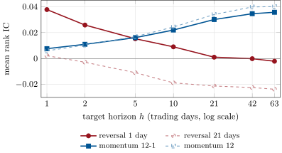
On the synthetic market the last month’s own return has an IC of $+0.0285$ with the next month (the reversal feature’s $-0.0285$ with the sign changed): continuation, so the full year wins. In the US data of Jegadeesh (1990) the last month reverses, and the skip wins. Figure 7.1 shows each feature’s IC against the length of its target: the one-day reversal is spent within a week, momentum keeps accumulating for three months.

Mean rank IC of four return features against returns over the next h days on the synthetic market, scored every day. The one-day reversal peaks at a day and is gone after two weeks; the last month’s reversal is negative at every horizon (the month continues); momentum rises to about 0.04 at a quarter, slightly higher without the skip. Data: firm.synthmkt, seed 1. — **Figure 7.1.** Mean rank IC of four return features against returns over the next $h$ days on the synthetic market, scored every day. The one-day reversal peaks at a day and is gone after two weeks; the last month’s reversal is negative at every horizon (the month continues); momentum rises to about 0.04 at a quarter, slightly higher without the skip. Data: `firm.synthmkt`, seed 1.

7.2 Volatility and range

Definition 7.3 (Range-based volatility estimator)

A range-based volatility estimator estimates a day’s return variance from its open, high, low and close prices rather than from close-to-close returns alone.

Definition 7.4 (Parkinson, Garman–Klass and Yang–Zhang estimators)

With $H, L, O, C$ a day’s high, low, open and close, the Parkinson estimator of the daily variance is $(\ln H/L)^2/(4\ln 2)$ ; the Garman–Klass estimator is $\tfrac12(\ln H/L)^2 - (2\ln 2 - 1)(\ln C/O)^2$ ; the Rogers–Satchell estimator is $\ln(H/C)\ln(H/O) + \ln(L/C)\ln(L/O)$ . The Yang–Zhang estimator over $n$ days adds the sample variance of overnight returns, $k$ times that of open-to-close returns and $1 - k$ times the average Rogers–Satchell term, with $k = 0.34/(1.34 + (n+1)/(n-1))$ .

For a Brownian motion without drift observed continuously, $\E[(\ln H/L)^2] = 4\ln2\,\sigma^2$ , which is Parkinson’s normalisation (Parkinson, 1980); the range carries much more information about $\sigma$ than the close alone. Each later estimator repairs a weakness of the one before. Garman and Klass (1980) combine the range with the open-to-close return; Rogers and Satchell (1991) are unbiased whatever the drift; Yang and Zhang (2000) add the overnight gap, which no intraday range can see.

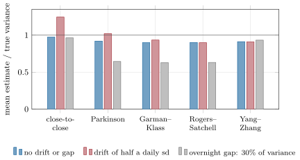
The chapter’s simulation of 4 000 days of one-minute Brownian paths scores them (Figure 7.2). Without drift or gaps, the variance of the Parkinson estimator is 5.2 times smaller than that of the squared close-to-close return, Garman–Klass’s 7.6 times, Rogers–Satchell’s 5.7 times; Yang–Zhang over twenty days is 7.5 times more efficient than the twenty-day close-to-close variance. Every range estimator is about 8–10% low, because a range observed at 390 points is narrower than the continuous one: discrete monitoring is a bias the formulas do not know about. A drift of half a standard deviation per day inflates the squared close-to-close return by 25% and Parkinson by 2%, leaves Rogers–Satchell and Yang–Zhang unchanged; an overnight gap carrying 30% of the variance makes the three single-day range estimators see only 63–64% of it, and only Yang–Zhang recovers the total.

Figure 7.2. Mean of each daily variance estimator relative to the true diffusion variance, on 4 000 simulated days of 390 one-minute steps. All range estimators read 8–10% low from discrete monitoring; a drift inflates close-to-close and Parkinson; an overnight gap is invisible to the single-day range estimators and recovered by Yang–Zhang. Data: the chapter’s module, seeded.

7.3 Volume and liquidity

Definition 7.5 (Volume surprise, Amihud illiquidity, turnover ratio)

The volume surprise of a security on a day is the logarithm of its volume divided by its average volume over a preceding window. Amihud illiquidity is the average over a window of the absolute daily return divided by the day’s traded value: the price move per unit of money traded (Amihud, 2002). The turnover ratio is traded volume divided by shares outstanding, averaged over a window.

Volume features measure attention and liquidity, and each has a claim behind it. Gervais, Kaniel and Mingelgrin (2001) found that stocks with unusually high volume over a day or a week tend to rise over the following month (the high-volume return premium): volume draws attention and investors’ attention moves prices. Amihud’s measure is a cheap proxy for price impact, and illiquid stocks are expected to pay a premium for bearing it. None of these mechanisms is in the book’s simulator, whose volume follows the size of each day’s move and the volatility state but carries no information about future returns; the table shows exactly that. A researcher who wants to study them needs real data, or a simulator that plants them.

7.4 Technical families as linear filters

Definition 7.6 (Moving-average crossover, linear filter)

A moving-average crossover with windows $n < m$ is the logarithm of the ratio of the average of the last $n$ prices to the average of the last $m$ prices; the classic rule is long when it is positive. A linear filter of returns is a predictor of the form $\sum_{j \ge 0} w_jr_{t-j}$ with fixed weights $w_j$ .

Proposition 7.7 (A crossover is a filter of past returns)

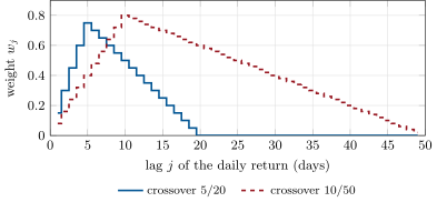
To first order in the returns, $\ln(\overline P_n/\overline P_m) = \sum_{j=0}^{m-2} w_jr_{t-j}$ with $w_j = \frac{(m - 1 - j)}{m} - \frac{(n - 1 - j)^+}{n}$ , where $r_{t-j}$ is the log return of $j$ days ago: the weights rise linearly over the short window, then fall linearly to zero at the long window’s length, and sum to $\frac{m - n}{2}$ .

Proof. The log of an average of prices is, to first order, the average of the log prices. The average of the last $n$ log prices is $\ln P_t - \sum_{j<n-1}\frac{n-1-j}{n}r_{t-j}$ , since the price $k$ days ago is $\ln P_t$ minus the $k$ most recent returns. Subtract the same expression with $m$ . The weights sum to $\frac{m-1}{2} - \frac{n-1}{2}$ . ∎

A crossover is therefore a momentum signal with a triangular window that skips most of the last $n$ days (Figure 7.3), and its apparent variety is a variety of weights on past returns. Brock, Lakonishok and LeBaron (1992) tested moving-average and trading-range rules on the Dow Jones index from 1897 to 1986 and found strong support for them; the filter view says what such a finding is about: the autocorrelation of index returns at the lags the weights emphasise. On the synthetic market, the 5/20 crossover has an IC of 0.022 at a month ( $t = 2.4$ ), a smoothed version of the momentum the simulator plants.

Weights a moving-average crossover puts on each past daily return (): rising over the short window, then falling linearly to zero at the long window. The 5/20 crossover sums to 7.5 and peaks at lag 5; the 10/50 to 20 and peaks at lag 10. — **Figure 7.3.** Weights a moving-average crossover puts on each past daily return (Proposition 7.7): rising over the short window, then falling linearly to zero at the long window. The 5/20 crossover sums to 7.5 and peaks at lag 5; the 10/50 to 20 and peaks at lag 10.

7.5 Predictor cards

Predictor card 7.1 — Momentum 12-1

Definition. $s_{i,t} = \prod_{k=t-251}^{t-21}(1 + r_{i,k}) - 1$ : the return from 252 to 21 trading days ago, ranked.

Inputs and timestamps. Daily closes up to 21 days before the decision date; delisting returns included.

Rationale. Underreaction to information and slow diffusion; the last month is skipped because it reverses in US data (Jegadeesh, 1990).

Horizon and half-life. One to three months. On the synthetic market the IC with a single day’s return is 0.0076 the next day and about 0.004 six months later; an exponential fit gives a half-life of 260 days.

Normalisation. Cross-sectional rank; neutralised to industries when industry momentum is not wanted.

Failure modes. Momentum crashes after market rebounds (Book 8); crowding; turnover costs.

Sources. Jegadeesh and Titman (1993); rs_features.lag_profile and half_life.

Predictor card 7.2 — Volume surprise

Definition. $s_{i,t} = \ln\bigl(V_{i,t}/\tfrac1{21}\sum_{k=1}^{21}V_{i,t-k}\bigr)$ , ranked.

Inputs and timestamps. Daily volumes to the close of $t$ (consolidated volume is known after the close).

Rationale. Unusual volume attracts attention and buyers; the high-volume return premium (Gervais, Kaniel and Mingelgrin, 2001).

Horizon and half-life. A month in the literature. Not measurable on the synthetic market, which plants no volume effect: its IC is 0.0009 ( $t = 1.3$ ) at a day and zero after.

Normalisation. Rank; the average excludes the current day.

Failure modes. Volume on news carries the news’ direction, not attention; index-rebalance and option-expiry days inflate volume mechanically.

Sources. Gervais, Kaniel and Mingelgrin (2001); the chapter’s table.

7.6 Tutorial: the feature library

Goal. Compute the chapter’s twelve features on the synthetic market, prove that none reads the future, and fill the IC table. End state: the table; Figures 7.1, 7.2 and 7.3.

Windows without look-ahead. Every rolling statistic is built from cumulative sums: row $t$ uses rows $t - w + 1$ to $t$ , and a window with a missing value is missing.

def _rolling_sum(x: np.ndarray, w: int) -> np.ndarray:
    """Sum of the last w rows (NaN until w rows exist or if any is NaN)."""
    x = np.asarray(x, float)
    cs = np.concatenate([np.zeros((1,) + x.shape[1:]), np.cumsum(np.nan_to_num(x), axis=0)])
    miss = np.concatenate([np.zeros((1,) + x.shape[1:]), np.cumsum(np.isnan(x), axis=0)])
    out = np.full(x.shape, np.nan)
    out[w - 1:] = cs[w:] - cs[:-w]
    bad = np.zeros(x.shape, bool)
    bad[w - 1:] = (miss[w:] - miss[:-w]) > 0
    out[bad] = np.nan
    return out


def _shift(x: np.ndarray, k: int) -> np.ndarray:
    out = np.full(x.shape, np.nan)
    if k == 0:
        return np.array(x, float)
    out[k:] = x[:-k]
    return out


def past_return(ret, window: int, skip: int = 0) -> np.ndarray:
    lr = np.log1p(np.asarray(ret, float))
    return np.expm1(_shift(_rolling_sum(lr, window), skip))

Listing 7.1. Rolling sums, shifts and past returns. code/firm/features/firm_features.py

The leakage test. Perturb every input after a cut-off and require the feature up to the cut-off to be unchanged; the acceptance tests run it on every feature, and on a feature that peeks, which it must catch.

def leakage_test(feature, inputs: tuple, cut: int, seed: int = 0) -> bool:
    """Apply `feature(*inputs)`, then again with every row after `cut` of every input multiplied by random factors;
    rows 0..cut of the output must be identical (NaN where NaN)."""
    rng = np.random.default_rng(seed)
    a = feature(*inputs)
    pert = []
    for x in inputs:
        y = np.array(x, float, copy=True)
        y[cut + 1:] = y[cut + 1:] * rng.uniform(0.5, 1.5, y[cut + 1:].shape)
        pert.append(y)
    b = feature(*pert)
    return bool(np.array_equal(np.nan_to_num(a[: cut + 1], nan=-9e9), np.nan_to_num(b[: cut + 1], nan=-9e9)))

Listing 7.2. The leakage test. code/firm/features/firm_features.py

Run ic_table(), ic_by_horizon for the four return features, range_race for the three cases and fig_features.py.

What to change next. Add long-term reversal (the return from five years to one year ago) and check its IC; replace the simulated minute paths by a firm.tape day and compare the range estimators on a price with a bid–ask bounce.

7.7 Build: the feature library

Purpose. The miniature firm’s standard bar features, computed one way everywhere, with a test that none of them looks ahead.

Interface. past_return(ret, window, skip), rolling_vol, ewma_vol, parkinson, garman_klass, rogers_satchell, yang_zhang, volume_surprise, amihud, turnover, ma_crossover, crossover_weights, leakage_test(feature, inputs, cut).

Rules. Panels (dates, names); row $t$ of an output uses input rows up to $t$ only; windows with a missing value are missing; volume averages exclude the current day.

Acceptance tests. code/firm/features/tests/: past returns with a skip; every feature passes the leakage test and a peeking feature fails it; range estimators within 10% of the true variance of a simulated Brownian day; the crossover equals its filter to first order.

Stretch. Intraday features from firm.tape bars; features on volume-clock bars (chapter 2); a registry that records each feature’s window and knowledge time for the predictor card.

Sources and further reading

N. Jegadeesh, “Evidence of predictable behavior of security returns”, Journal of Finance 45(3), 1990; N. Jegadeesh and S. Titman, “Returns to buying winners and selling losers”, Journal of Finance 48(1), 1993.
W. F. M. De Bondt and R. Thaler, “Does the stock market overreact?”, Journal of Finance 40(3), 1985.
M. Parkinson, “The extreme value method for estimating the variance of the rate of return”, Journal of Business 53(1), 1980; M. B. Garman and M. J. Klass, “On the estimation of security price volatilities from historical data”, Journal of Business 53(1), 1980.
L. C. G. Rogers and S. E. Satchell, “Estimating variance from high, low and closing prices”, Annals of Applied Probability 1(4), 1991; D. Yang and Q. Zhang, “Drift-independent volatility estimation based on high, low, open, and close prices”, Journal of Business 73(3), 2000.
Y. Amihud, “Illiquidity and stock returns: cross-section and time-series effects”, Journal of Financial Markets 5(1), 2002; S. Gervais, R. Kaniel and D. H. Mingelgrin, “The high-volume return premium”, Journal of Finance 56(3), 2001.
W. Brock, J. Lakonishok and B. LeBaron, “Simple technical trading rules and the stochastic properties of stock returns”, Journal of Finance 47(5), 1992.

7.8 Exercises

Exercise 7.1 ★

A stock’s day has $H = 51.20$ , $L = 49.80$ . What daily volatility does the Parkinson estimator give?

Solution

Solution of Exercise 7.1.

$\ln(51.20/49.80) = 0.0277$ ; $(0.0277)^2/(4\ln2) = 0.000277$ , a daily volatility of 1.67%.

Exercise 7.2 ★

Monthly returns of 2%, $-1\%$ , 4% and 3% (oldest first). What is the 3-1 momentum feature at the end of the fourth month, and the four-month return?

Solution

Solution of Exercise 7.2.

3-1 momentum skips the last month: $1.02 \times 0.99 \times 1.04 - 1 = 5.02\%$ . The four-month return is $1.050 \times 1.03 - 1 = 8.17\%$ .

Exercise 7.3 ★

A stock trades USD 40 million a day and moves 1.2% on average in absolute value. What is its Amihud illiquidity, in percent per USD million? And a stock trading USD 2 million that moves 2.5%?

Solution

Solution of Exercise 7.3.

$1.2\%/40 = 0.03\%$ per USD million; $2.5\%/2 = 1.25\%$ per USD million, about 40 times less liquid by this measure.

Exercise 7.4 ★★

Compute the weights of the 3/6 crossover by Proposition 7.7, and their sum.

Solution

Solution of Exercise 7.4.

$w_j = (5 - j)/6 - (2 - j)^+/3$ : $w_0 = 1/6$ , $w_1 = 1/3$ , $w_2 = 1/2$ , $w_3 = 1/3$ , $w_4 = 1/6$ ; the sum is $1.5 = (6 - 3)/2$ .

Exercise 7.5 ★★

The Parkinson estimator is 5.2 times as efficient as a squared daily return. How many days of Parkinson estimates give a daily-variance estimate as precise as sixty days of squared close-to-close returns?

Solution

Solution of Exercise 7.5.

The variance of an average falls with the number of days, so $60/5.2 = 11.5$ days of Parkinson estimates match sixty squared returns.

Exercise 7.6 ★★

By Proposition 7.2, with standard deviations of the 12-1 part and of the last month’s return in the ratio $\sqrt{11}:1$ , ICs of 0.03 for the first and $-0.03$ for the second, and the two parts uncorrelated, what is the IC of the full twelve-month return?

Solution

Solution of Exercise 7.6.

$(\sqrt{11} \times 0.03 + 1 \times (-0.03))/\sqrt{12} = (0.0995 - 0.03)/3.464 = 0.020$ , a third less than the 0.03 of the 12-1 part alone: with a monthly reversal, the skip is worth a third of the IC.

Exercise 7.7 ★★★

Coding. Rerun range_race with 30 steps a day instead of 390. How large does the discrete-monitoring bias of Parkinson become, and why?

Solution

Solution of Exercise 7.7.

With 30 steps the range estimators read 22–30% low (Parkinson 0.78, Garman–Klass and Rogers–Satchell 0.70) against 8–10% with 390: the true high and low fall between the sampled points more often and by more when the points are sparser. Bars built from few trades (illiquid stocks) have the same problem.

Exercise 7.8 ★★★

Find the flaw. “Our volume-surprise predictor divides today’s volume by the average volume of the 21 days centred on today, so that it is not biased by trends in volume.”

Solution

Solution of Exercise 7.8.

A window centred on today includes the next ten days’ volume, which is not known at the close: the feature looks ahead. The leakage test would catch it. Use the preceding 21 days, excluding today.

7.9 Problem: The Range-Estimator Race

Problem 7.1

Weekend problem — which daily variance estimator to trust, and when

The chapter’s simulation: 4 000 days, 390 one-minute Brownian steps a day, a daily volatility of 1%, seed 5; in turn no drift and no gap, a drift of half a daily standard deviation, and an overnight gap carrying 30% of the daily variance.

Part I — The formulas.

Why is Parkinson’s constant $4\ln2$ ?
Which estimator needs only the high and the low?
Which is unbiased whatever the drift, and why?
What does Yang–Zhang add, and what does its weight $k$ equal for twenty days?

Part II — Efficiency.

What are the efficiencies of Parkinson, Garman–Klass and Rogers–Satchell relative to the squared close-to-close return?
And of twenty-day Yang–Zhang relative to the twenty-day close-to-close variance?
How many days of close-to-close returns does one day of Garman–Klass replace?

Part III — Bias.

What are the four range estimators’ biases without drift or gap, and what causes them?
What does the drift do to close-to-close, to Parkinson and to Rogers–Satchell?
What does the gap do to the three single-day range estimators, and to Yang–Zhang?
Why does the close-to-close estimator suffer from the drift but not from the gap?
How would a bid–ask bounce in the high and low affect the range estimators?

Part IV — Choice.

For a stock with large overnight gaps, which estimator?
For a 24-hour market with no gap and strong intraday trends, which?
For a volatility feature that must be computed from daily closes only, which, and at what cost?
What would you check before using a range estimator on real data?
Why do the efficiency gains matter for a volatility predictor?
State the named result: the efficiencies of the four range estimators and the share of variance the single-day ones miss with a 30% gap.
Which of the chapter’s features use a volatility estimate?
In one sentence: what does the range know that the close does not?

Solution

Solution of Problem 7.1.

1. For a Brownian motion observed continuously, the expected squared range of its logarithm over a day is $4\ln2\,\sigma^2$ . 2. Parkinson. 3. Rogers–Satchell: each of its two products pairs a high (or low) measured from the close and from the open, so a drift enters with opposite signs and cancels. 4. The overnight variance; $k = 0.34/(1.34 + 21/19) = 0.139$ . 5. 5.2, 7.6 and 5.7. 6. 7.5. 7. About 7.6. 8. 0.92, 0.90, 0.90 and 0.91: the range seen at 390 points is narrower than the continuous one. 9. Close-to-close rises to 1.25 (it measures $\sigma^2 + \mu^2$ ), Parkinson to 1.02, Rogers–Satchell stays at 0.90. 10. The single-day range estimators fall to 0.63–0.64; Yang–Zhang stays at 0.93. 11. The close-to-close return spans the night, so it contains the gap, and the drift adds $\mu^2$ to its second moment. 12. Highs at the ask and lows at the bid widen the range and bias every range estimator upwards, more for liquid-looking but wide-spread stocks. 13. Yang–Zhang. 14. Rogers–Satchell (or Yang–Zhang with its overnight part near zero). 15. Close-to-close (an EWMA of squared returns), with five to eight times more days for the same precision. 16. That highs and lows exclude erroneous prints and auction prints, that the bars cover the whole session, and how wide the spread is. 17. A less noisy volatility makes a better volatility predictor and better risk scaling of other predictors. 18. Named result: relative to squared close-to-close returns, Parkinson is 5.2 times as efficient, Garman–Klass 7.6 and Rogers–Satchell 5.7, and twenty-day Yang–Zhang 7.5 times the twenty-day close-to-close variance; with an overnight gap carrying 30% of the variance the single-day range estimators see 63–64% of it. 19. Low volatility and Amihud illiquidity (through absolute returns), and any feature scaled by volatility. 20. The path: how far the price travelled during the day, not only where it ended.

7.10 Interview questions

Interview question 7.1 ★ researcher, trader

Why do momentum signals skip the most recent month?

Solution

Solution of Interview question 7.1.

Because the most recent month’s return tends to reverse (a negative first-order autocorrelation of monthly returns), so it works against the continuation that momentum bets on; skipping it removes a component with the wrong sign. In a market without that reversal the skip would cost information.

What the interviewer is looking for: the reversal as the reason, not “convention”.

Interview question 7.2 ★★ researcher, risk

How would you estimate a stock’s daily volatility from one month of daily bars as precisely as possible?

Solution

Solution of Interview question 7.2.

Use the range: Garman–Klass or, with overnight gaps, Yang–Zhang, over the month, after cleaning highs and lows of bad prints; each is five to eight times more efficient than squared close-to-close returns, and Yang–Zhang handles drift and gaps. Correct for the downward bias of a discretely observed range if the bars are thin.

What the interviewer is looking for: range estimators, their efficiency and their failure cases.

Interview question 7.3 ★★ researcher

Show that a moving-average crossover is a weighted sum of past returns. What weights?

Solution

Solution of Interview question 7.3.

The log of an average of prices is, to first order, an average of log prices, and each log price is today’s minus a sum of recent returns. The difference of the two averages gives $w_j = (m - 1 - j)/m - (n - 1 - j)^+/n$ : triangular weights rising over the short window and falling to zero at the long one.

What the interviewer is looking for: the first-order derivation and the shape of the weights.

Interview question 7.4 ★★ developer, mle

How do you test automatically that a feature pipeline never uses future data?

Solution

Solution of Interview question 7.4.

A perturbation test: recompute every feature after multiplying all inputs after a cut-off by random factors, and require identical outputs up to the cut-off, for many cut-offs; plus a feature that deliberately peeks, to prove the test catches it. Also a data-access layer that refuses data after the decision time.

What the interviewer is looking for: an automated, falsifiable test.

Interview question 7.5 ★★ researcher, trader

What does Amihud’s illiquidity measure capture, and what are its weaknesses?

Solution

Solution of Interview question 7.5.

The price move per unit of money traded, a proxy for price impact. Weaknesses: it is noisy day by day (a single large move dominates), mixes news-driven moves with impact, depends on price level through the traded value, and is zero on days without trading.

What the interviewer is looking for: what it proxies and why it is noisy.

Interview question 7.6 ★★★ researcher

A new feature has an IC of zero on your simulator and 0.02 on real data. What do you conclude about the feature, and about the simulator?

Solution

Solution of Interview question 7.6.

The feature may carry real information that the simulator does not contain: a simulator only reproduces the effects planted in it. Nothing is learned about the feature from the simulator; the real-data result must be tested like any other (search, overlap, costs), and the simulator’s scope is clarified: it cannot validate that feature’s effect.

What the interviewer is looking for: a simulator’s scope, and not treating it as evidence against a real effect.

Terms defined in this chapter

See all 2333 terms in the glossary