Research Craft: Predictors, Backtests, Measurement, Portfolios · Research
21Live Experiments
A new execution algorithm handles ten per cent of the firm’s orders for two weeks, 2 485 of 24 000, and saves 0.55 basis point of implementation shortfall on average, with a standard error of 0.48. The 95% interval runs from to 0.39: the experiment cannot tell a saving from a cost. At half the flow it would need 77 trading days to detect a saving of 0.3 basis point, and 38 with the variance reduction of this chapter. Even a perfect answer would be to a narrower question than the desk’s: in the chapter’s simulated flow the new algorithm saves 0.30 basis point on its own orders but adds 0.25 to the firm’s other orders in the same stock, side and day, so that switching everything over saves 0.08. Research reaches production through paper trading, canaries and staged rollouts, and is then measured on live flow; this chapter covers both, with firm.abtest.
21.1 Paper trading and shadow mode
Definition 21.1 (Paper trading)
Paper trading runs a new strategy in real time on live market data: it computes its signals and generates its orders, which are recorded and checked but never sent, and fills them with a fill model.
Paper trading tests everything that does not depend on the market’s reaction. The live feeds arrive with their real timing and gaps; the signals computed live can be compared with the same signals recomputed by the research code on the same data, value by value; the orders pass or fail the pre-trade risk checks; the strategy lives through the operational calendar (start-up and shutdown, corporate actions, holidays, the index rebalance) that a backtest compresses into rows. What paper trading cannot test is the fills. It is a simulator running on live data, with the blind spots of every simulator: chapter 19 showed that a replay without the strategy’s own orders misses the trades that stopped at them and the levels where they were alone. Shadow trading (chapter 19) compares the simulator with the live trading of an existing strategy; paper trading is the stage before a new strategy has any.
The exit condition of paper trading is therefore not its P&L. It is parity: live signals equal to the research signals within a stated tolerance, every order it would have sent accepted by the risk checks, and a full operational cycle crossed without manual repair. A strategy whose paper P&L is good and whose live signals differ from research has not been tested; it has been replaced by another one.
21.2 Canaries and staged rollouts
Definition 21.2 (Canary deployment, staged rollout)
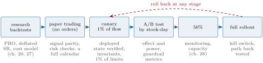
A canary deployment runs a new version of a trading component on a small share of the production flow (the canary) alongside the old version, and compares the two before the new one receives more. A staged rollout expands the share in steps (for instance 1%, 10%, 50%, 100%), each step gated by stated checks, with a tested path back to the old version at every step.
The most expensive deployment failure in the public record was a staged deployment. From 27 July 2012 Knight Capital placed new order-routing code on a limited number of servers on successive days, ahead of a new NYSE programme starting on 1 August. A technician did not copy the new code to one of the eight servers; no second person reviewed the deployment, and no written procedure required it. On 1 August the eighth server ran an old, defective function that the new code’s repurposed flag reactivated: for 212 incoming parent orders it sent millions of child orders, 4 million executions in 154 stocks for more than 397 million shares in about 45 minutes. Knight was left with a net long position of about $3.5 billion in 80 stocks and a net short of about $3.15 billion in 74, and realised a loss of $460 million. Before the open, its systems had sent 97 automated e-mails citing the old function by name; they were not designed as alerts and nobody read them. The SEC’s order of October 2013 imposed a $12 million penalty.
Three lessons follow, none of them statistical. A stage is only as good as its check of the deployed state: every server, process and configuration runs the version the stage says it runs. An alert is a message designed and routed to be acted on, not a log line that happens to be e-mailed. And a stage must be capped in what it can do: a canary with 1% of the flow must hold 1% of the risk limits, and invariants such as “child quantity never exceeds the parent’s” must be checked on every order, where they fire on the first violation. The statistical comparison of canary and control is for a different class of defect.
Proposition 21.3 (How long a statistical canary takes)
A canary receives a share of a flow; a defect adds to a per-order metric of standard deviation ; the alarm is a one-sided -test of the canary’s mean against the control’s at threshold . The expected alarm comes after about
canary orders: nearly independent of the share when it is small.
Proof. After canary orders the control has , and the difference of means has variance . The expected statistic reaches at the stated . ∎
With the chapter’s flow ( basis points, 2 400 orders a day), a defect costing 5 basis points an order and an alarm at , a 1% canary raises the alarm after 194 damaged orders and 8.1 days, a 10% canary after 214 orders and 0.89 day, a 50% canary after 385 orders and 0.32 day. A smaller canary does not reduce the damage done before a statistical alarm; it spreads it over more time. What a small canary buys is a small exposure for defects caught by invariants and limits, and time for people to look.
21.3 Randomised A/B tests on live flow
Definition 21.4 (A/B test, randomisation unit, interference, sample ratio mismatch)
An A/B test compares two versions of a component by assigning units of live flow to them at random and comparing an outcome. The randomisation unit is what is assigned: an order, a stock-day, a day, a client. Interference occurs when the outcome of one unit depends on the assignment of others, so that the difference between the arms of a test differs from the effect of switching every unit. A sample ratio mismatch (SRM) is an observed split between the arms that differs, beyond chance, from the planned one (Fabijan and co-authors).
The chapter’s simulated flow has 2 400 parent orders a day in 500 stocks, drawn with popularity inversely proportional to rank. An order’s implementation shortfall, in basis points against its arrival price, is the firm’s pre-trade cost estimate (standard deviation 6.9 across orders), the estimate’s error, the beta-adjusted market move over the order’s scheduled window signed by its side, idiosyncratic noise, and a day effect common to all orders; the mean is 11.7 and the standard deviation 23.1. The new algorithm saves 0.30 basis point on each order it handles, and adds 0.25 to the other orders of the same stock, side and day when all of them are on the new algorithm (it trades earlier in the window and leaves its siblings more impact).
Assignment. firm.abtest.assign hashes the unit’s identifier with the experiment’s name and compares the first eight bytes of the SHA-256 digest, read as a fraction, with the planned share. The assignment is deterministic (the same order always goes to the same arm, on every server, without a shared table), independent across experiments with different names, and reproducible afterwards by anyone holding the identifiers. In the two-week experiment of the opening, 2 485 of 24 000 orders went to the new algorithm against a planned 2 400: , a p-value of 0.07, no mismatch at 5%. A mismatch would not be a statistical curiosity: it is the symptom of orders lost, duplicated or re-routed in one arm, and it invalidates the comparison until explained.
Interference. In the flow, 88% of orders share their stock, side and day with another of the firm’s orders. When orders are randomised one by one, a treated order and a control order have, on average, the same share of treated siblings, so the difference between the arms measures the direct saving, . The desk’s question is what happens when every order moves: . A randomisation unit must contain the interference: here the stock-day, all of a stock’s orders on a day in the same arm. The day itself contains every interference within a day, but offers only one unit a day, and the day effect is then the noise; alternating the treatment through time in this way is a switchback design (Bojinov, Simchi-Levi and Zhao), common where units interfere, at the price of few units and of carryover from one period to the next.
def cluster_diff(y, t, cluster):
    """Order-weighted difference in means when whole clusters are assigned, with a cluster-robust standard error:
    each arm's mean is a ratio of cluster totals, linearised per cluster."""
    y, t, cluster = np.asarray(y, float), np.asarray(t, bool), np.asarray(cluster)
    _, inv = np.unique(cluster, return_inverse=True)
    n = np.bincount(inv).astype(float)
    tot = np.bincount(inv, weights=y)
    arm = np.bincount(inv, weights=t) / n
    if np.any((arm > 0) & (arm < 1)):
        raise ValueError("an arm must be constant within each cluster")
    mean, var = [], 0.0
    for m in (arm > 0.5, arm < 0.5):
        mu = tot[m].sum() / n[m].sum()
        e = tot[m] - mu * n[m]
        k = int(m.sum())
        mean.append(mu)
        var += k / (k - 1) * float((e * e).sum()) / n[m].sum() ** 2
return float(mean[0] - mean[1]), math.sqrt(var)21.4 Variance reduction
Definition 21.5 (CUPED)
CUPED (controlled experiments using pre-experiment data; Deng, Xu, Kohavi and Walker) compares the arms on the adjusted outcome , where are covariates the treatment cannot affect and is the coefficient of the regression of on pooled over both arms.
Proposition 21.6 (What CUPED buys)
The adjusted difference in means is unbiased for the treatment effect, and its variance is the unadjusted variance times , where is the share of the outcome’s variance explained by the covariates.
Proof. Randomisation gives the covariates the same distribution in both arms, so and the adjustment removes nothing from the expected difference. The variance of is smallest at the regression coefficient, where it is ; the difference of two independent means inherits the factor. Estimating on the pooled data changes this by a term of order . ∎
The covariates must be fixed before assignment or lie outside the firm’s reach. The pre-trade cost estimate qualifies, and explains 9% of the variance of the shortfall. So does the market’s beta-adjusted move over the order’s scheduled window: the portfolio manager fixes the window before the order is assigned, and the market does not move because one of the firm’s algorithms rather than the other is working it. With both covariates is 0.51, close to the halving Deng and co-authors reported for Bing’s experiments. The order’s realised duration, its fill rate or its participation do not qualify: the algorithm changes them, and adjusting for them removes part of the effect. Post-stratification (Miratrix, Sekhon and Yu) is CUPED with stratum indicators as covariates, nearly as efficient as assigning within strata in advance; for a design randomised by stock-day, analysing within each day (subtracting each day’s mean from outcome and covariates) is the stratification that removes the day effect.
Each design below was run as 100 simulated experiments of 60 days on half the flow (the mean estimate, the spread of the estimates, the mean reported standard error, and the days that standard error implies for 80% power on 0.3 basis point):
| design and estimator | estimate | spread | s.e. | days for 0.3 bp |
|---|---|---|---|---|
| by order: difference in means | 0.123 | 0.122 | 77 | |
| by order: stratified (pre-trade quintiles) | 0.119 | 0.117 | 72 | |
| by order: CUPED, pre-trade estimate | 0.121 | 0.116 | 70 | |
| by order: CUPED, pre-trade and market | 0.095 | 0.085 | 38 | |
| by day | 0.656 | 0.788 | 3 253 | |
| by stock-day | 0.235 | 0.235 | 290 | |
| by stock-day, within day | 0.188 | 0.184 | 178 | |
| by stock-day, within day, CUPED | 0.093 | 0.082 | 35 |
Every order-level design estimates the direct saving, ; every design that assigns whole stock-days or days estimates the rollout’s, (the day design’s is within its spread of 0.66). The reported standard errors match the spread of the estimates across experiments. CUPED with the market covariate halves the days needed; the pre-trade estimate alone and stratification on it buy little, because the estimate explains little. Randomising by day multiplies the days by 42. Randomising by stock-day and analysing within the day, with CUPED, is as precise as the best order-level design and answers the right question; the answer is small, and detecting a saving of 0.08 basis point at 80% power would take 503 trading days.
21.5 Sizing and stopping an experiment
Definition 21.7 (Minimum detectable effect, sequential test)
The minimum detectable effect of a design is the smallest true effect it detects with a stated power at a stated size. A sequential test examines the data as they arrive and may stop at any look, with its size controlled over all the looks it might take.
Proposition 21.8 (Minimum detectable effect and sample size)
For a two-sided test of size and power on an estimate with standard error , the minimum detectable effect is , which is at 5% and 80%. With outcome standard deviation and a share of units treated, detecting an effect needs
Proof. The test rejects when ; if this has probability (neglecting the other tail) when . Substitute . ∎
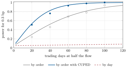
The standard deviation of 23.1 basis points and 2 400 orders a day give 77.7 days at half the flow for 0.3 basis point, and 38.2 with CUPED’s residual standard deviation of 16.2; the simulated experiments, rejecting in 78% of runs at 80 days without CUPED and 76% at 40 days with it, confirm the formula (Figure 21.2). The equal split minimises the sample size; a 10% experiment, as in the opening, needs times as many orders.
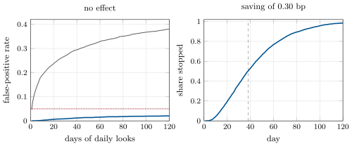
rs_abtest.Peeking. A desk watching an experiment’s dashboard every morning and stopping the first day its p-value falls below 5% runs a different test from the one the p-value describes. On 4 000 simulated experiments with no effect at all, a fixed-horizon test looked at once rejects in 5% of them; looked at every day, it rejects at least once in 29% within 38 days, 33% within 60 and 38% within 120 (Figure 21.3).
The mixture sequential probability ratio test, a descendant of Wald’s sequential test (1945), turns continuous monitoring into a valid procedure (Johari, Koomen, Pekelis and Walsh, who deployed it on a commercial testing platform). For an estimate with variance at the current look, and effects drawn from under the alternative, the mixture likelihood ratio against no effect is
Under no effect is a nonnegative martingale starting at 1, so the probability that it ever exceeds is at most (Ville’s inequality). The always-valid p-value is the running minimum of ; stopping whenever it falls below keeps the error at however often one looks. On the same null experiments it crossed 5% in 46, 62 and 82 of the 4 000 by days 38, 60 and 120. With the real saving of 0.30 and CUPED, and , half the experiments stop by day 38, the fixed horizon’s length, 4% by day 10 and 98% by day 120. A harmful change of basis point stops at a median of 6 days. The sequential test gives up a fixed end date; it keeps the size under monitoring and stops early when the effect is large, which is when stopping matters.
rs_abtest.peeking, stopping.The plan. Everything that decides the outcome is written down before the first order is assigned: the metric and its guardrails (fill rate, rejects, mark-outs), the randomisation unit, the share, the covariates, the horizon or the sequential rule with its , the minimum detectable effect, and what will be done at each outcome. Chapter 1’s research log records it; chapter 20’s arithmetic about trials applies to experiments as much as to backtests, and a desk that runs twenty experiments a year will see one false saving a year at 5%.
21.6 Tutorial: is the new algorithm better?
Goal. Simulate the firm’s order flow with a new execution algorithm, assign orders by hash, compare designs and estimators, size the experiment, and monitor it sequentially. End state: the table, Figures 21.2 and 21.3.
Assignment and estimation: the hash, the difference in means, CUPED.
def bucket(unit, experiment: str, salt: str = "") -> float:
    h = hashlib.sha256(f"{experiment}:{salt}:{unit}".encode()).digest()
    return int.from_bytes(h[:8], "big") / 2.0**64


def assign(units, experiment: str, share: float = 0.5, salt: str = "") -> np.ndarray:
    return np.array([bucket(u, experiment, salt) < share for u in units], dtype=bool)


def diff_means(y, t):
    y, t = np.asarray(y, float), np.asarray(t, bool)
    a, b = y[t], y[~t]
    d = a.mean() - b.mean()
    return float(d), math.sqrt(a.var(ddof=1) / len(a) + b.var(ddof=1) / len(b))


def cuped(y, X, t):
    """Regress y on the covariates pooled over both arms, then compare the adjusted outcomes. The covariates must be
    unaffected by the treatment (measured before assignment, or outside the firm's reach)."""
    y = np.asarray(y, float)
    X = np.asarray(X, float).reshape(len(y), -1)
    Xc = X - X.mean(axis=0)
    theta = np.linalg.lstsq(Xc, y - y.mean(), rcond=None)[0]
    d, se = diff_means(y - Xc @ theta, t)
    return d, se, theta
Listing 21.2. Hash assignment, the difference in means and CUPED. code/firm/abtest/firm_abtest.py - The flow:
rs_abtest.orders(days, seed, share, unit)draws the orders, their covariates, the siblings and the outcome;hook()runs the two-week, 10% experiment and its SRM check. - Designs:
calibration()runs 100 experiments per design;rollout()gives the true effect of switching everything. Sequential monitoring: the mixture likelihood ratio and the always-valid p-value.
def msprt(d, se, tau: float):
    """Lambda = sqrt(V / (V + tau^2)) exp(tau^2 d^2 / (2 V (V + tau^2))), V = se^2: the likelihood ratio of the
    estimate d under a N(0, tau^2) mixture of effects against the null of no effect."""
    d, V = np.asarray(d, float), np.asarray(se, float) ** 2
    return np.sqrt(V / (V + tau * tau)) * np.exp(tau * tau * d * d / (2 * V * (V + tau * tau)))


def always_valid_p(d, se, tau: float):
    return np.minimum.accumulate(np.minimum(1.0, 1.0 / msprt(d, se, tau)), axis=-1)
Listing 21.3. The mixture sequential probability ratio test. code/firm/abtest/firm_abtest.py - Run
peeking(),stopping()andfig_abtest.py.
What to change next. Make the new algorithm harm its siblings more than it helps itself (a spillover of 0.40) and see an order-level test approve a change that loses money; randomise by client instead of stock-day and ask what interference that contains.
21.7 Build: the experiment toolkit
Purpose. Every change to a trading component reaches full flow through a staged rollout, and every claimed improvement comes from a randomised experiment, analysed as planned.
Interface. bucket(unit, experiment, salt), assign(units, experiment, share, salt), diff_means(y, t), cuped(y, X, t), stratified(y, t, strata), cluster_diff(y, t, cluster), demean_by(v, group), power(effect, se, alpha), mde(se, alpha, power), sample_size(effect, sd, alpha, power, share), srm_pvalue(n_t, n_c, share), msprt(d, se, tau), always_valid_p(d, se, tau).
Rules. Assignment by hash of a stable identifier, never by a mutable table; covariates fixed before assignment; the randomisation unit contains the interference; the SRM check runs before any estimate is read; a fixed horizon is not looked at early, and a sequential rule is chosen before the start.
Acceptance tests. code/firm/abtest/tests/: a deterministic, balanced assignment, independent across experiments; CUPED’s variance falling by on a known covariate, stratification between the raw and adjusted estimates; cluster arms constant or an error; power, minimum detectable effect and sample size consistent; an always-valid p-value non-increasing and below 5% in fewer than 5% of 2 000 null streams of 200 looks, while daily looks at a fixed-horizon test exceed 30%.
Stretch. Variance-weighted estimators for unequal clusters; guardrail metrics with their own sequential tests; a switchback design with carryover.
Sources and further reading
- A. Deng, Y. Xu, R. Kohavi and T. Walker, “Improving the sensitivity of online controlled experiments by utilizing pre-experiment data”, WSDM, 2013.
- R. Kohavi, D. Tang and Y. Xu, Trustworthy Online Controlled Experiments, Cambridge University Press, 2020.
- A. Fabijan et al., “Diagnosing sample ratio mismatch in online controlled experiments”, KDD, 2019.
- R. Johari, P. Koomen, L. Pekelis and D. Walsh, “Always valid inference: continuous monitoring of A/B tests”, Operations Research 70(3), 2022 (and “Peeking at A/B tests”, KDD, 2017).
- A. Wald, “Sequential tests of statistical hypotheses”, Annals of Mathematical Statistics 16(2), 1945.
- SEC, In the Matter of Knight Capital Americas LLC, Release No. 34-70694, 16 October 2013.
- I. Bojinov, D. Simchi-Levi and J. Zhao, “Design and analysis of switchback experiments”, Management Science 69(7), 2023.
- L. W. Miratrix, J. S. Sekhon and B. Yu, “Adjusting treatment effect estimates by post-stratification in randomized experiments”, Journal of the Royal Statistical Society B 75(2), 2013.
21.8 Exercises
Exercise 21.1 ★
The two-week experiment estimates a saving of 0.55 basis point with a standard error of 0.48. Give the 95% interval and the verdict.
Solution
Solution of Exercise 21.1.
: from to 0.39. The interval contains zero and savings three times larger than any plausible one: the experiment is uninformative, not negative. It needed more orders, a larger share, or CUPED.
Exercise 21.2 ★
The same experiment planned 10% of 24 000 orders and assigned 2 485. Compute the SRM statistic and its p-value. What would you do with a p-value of 0.0001?
Solution
Solution of Exercise 21.2.
, a two-sided p-value of 0.07: no mismatch at 5%. At 0.0001, stop reading the estimate and find the cause (orders dropped, duplicated or re-routed in one arm, a filter applied after assignment, a server running an old assignment rule); the comparison is not valid until the split is explained.
Exercise 21.3 ★
An estimate’s standard error is 0.085 basis point. What is the minimum detectable effect at 5% and 80%, and what is the power against a true saving of 0.3?
Solution
Solution of Exercise 21.3.
basis point; the power against 0.3 is 0.94.
Exercise 21.4 ★★
Which of these may serve as CUPED covariates in an execution experiment: the pre-trade cost estimate; the market’s move over the order’s scheduled window; the order’s realised duration; the algorithm’s fill rate; the stock’s shortfall on the previous day? With covariates explaining 51% of the variance, how many of 77 days remain?
Solution
Solution of Exercise 21.4.
Allowed: the pre-trade estimate (fixed before assignment), the market’s move over the scheduled window (outside the algorithm’s reach), the stock’s previous-day shortfall (before assignment). Not allowed: the realised duration and the fill rate, which the algorithm changes; adjusting for them removes part of the effect. With the variance is multiplied by 0.49: days.
Exercise 21.5 ★★
A defect costs 5 basis points an order, the per-order standard deviation is 23.1, the alarm is at and the flow is 2 400 orders a day. How many orders and how long until the alarm with a 1% canary, a 10% one and a 50% one? What would have stopped Knight’s defect, and why is it not statistics?
Solution
Solution of Exercise 21.5.
: 194 orders and 8.1 days at 1%, 214 orders and 0.89 day (348 minutes of a 6.5-hour session) at 10%, 385 orders and 0.32 day at 50%. Knight’s defect sent child orders without regard to the parent’s filled quantity: an invariant (child quantity never exceeds the parent’s) checked on each order, a position limit sized to the stage, and a kill switch would have stopped it in seconds. A runaway order is a violated rule, not a small shift in a mean.
Exercise 21.6 ★★
With a direct saving of 0.30, a spillover of 0.25 onto fully treated siblings and 88.3% of orders with siblings, what is the effect of the full rollout? Why does randomising by order measure 0.30, and which unit measures the rollout?
Solution
Solution of Exercise 21.6.
, about . Randomised order by order, treated and control orders have the same expected share of treated siblings, so the spillover is the same in both arms and cancels in the difference. The stock-day (all of a stock’s orders on a day in one arm) contains the interference, and measures the rollout.
Exercise 21.7 ★★★
Coding. Run rs_abtest.stopping under the real saving with and as well as 0.3. Report the median stopping days and explain why both a small and a large are slower.
Solution
Solution of Exercise 21.7.
Median stopping days: 56 with , 38 with , 44 with . A small puts the alternative’s mass on effects too small to distinguish quickly; a large one spreads it over effects much larger than 0.3 and pays a factor for them. The best is near the effect one expects.
Exercise 21.8 ★★★
Find the flaw. “We checked the experiment’s dashboard every morning, and on day 23 the p-value fell to 0.04, so we stopped and rolled the new algorithm out: a significant saving at 5%.”
Solution
Solution of Exercise 21.8.
Daily looks at a fixed-horizon test with no effect at all reach at some look within 23 days in 25% of experiments, not 5%. Either fix the horizon and look once, or use an always-valid p-value (the mixture sequential test), whose size holds at every look.
21.9 Problem: Is the New Algorithm Better?
Problem 21.1
Weekend problem — an execution experiment, designed and read
The chapter’s simulated flow: 2 400 orders a day, a new algorithm saving 0.30 basis point on its own orders and costing its siblings 0.25.
Part I — The design.
- What are the mean and standard deviation of an order’s shortfall, and what are its components?
- What properties does hash assignment give, and why do they matter on a trading system?
- Check the opening experiment’s split.
- What does randomising by order measure, and what does the full rollout save?
- What should Knight’s staged deployment have checked at each stage?
Part II — Precision.
- How many days at half the flow does the difference in means need for 0.3 basis point?
- Which covariates does CUPED use, what is their , and how many days remain?
- What do the pre-trade estimate and stratification on it buy, and why so little?
- What does randomising by day cost?
- How precise is the stock-day design analysed within the day with CUPED, and what does it estimate?
Part III — Stopping.
- What false-positive rates does daily peeking at a fixed-horizon test give by days 38 and 60?
- How many of the 4 000 null experiments does the mixture sequential test stop by the same days?
- Under the real saving, when does the sequential test stop?
- How fast does it catch a harmful change of 1 basis point?
Part IV — The verdict.
- State the named result: the trading days needed to detect a 0.3 basis point improvement at 80% power, with and without CUPED.
- Is the new algorithm better?
- How would you roll it out?
- How long would a 1% canary take to notice a defect costing 5 basis points an order, and what would you rely on instead?
- What goes into the experiment’s plan before the first order?
- In one sentence: what does an A/B test on live flow measure?
Solution
Solution of Problem 21.1.
- Mean 11.7, standard deviation 23.1 basis points: the pre-trade estimate, its error, the signed market move over the window, idiosyncratic noise and a day effect.
- Deterministic, stateless, identical on every server, independent across experiments, reproducible afterwards: no shared table to fall out of sync.
- 2 485 against 2 400 planned: , p-value 0.07, no mismatch.
- The direct saving, ; the rollout saves .
- That every server ran the new code (a second review), that alerts reached someone, and that each stage’s limits and invariants capped what it could do.
- 77 days (the formula gives 77.7).
- The pre-trade estimate and the market’s move over the scheduled window; ; 38 days.
- 72 and 70 days: the pre-trade estimate explains only 9% of the variance.
- A spread of 0.66 and 3 253 days for 0.3 basis point: one unit a day, and the day effect is the noise.
- Spread 0.093 and 35 days for 0.3 basis point, like the best order-level design; it estimates the rollout’s , which would take 503 days to detect.
- 29% and 33%.
- 46 and 62 of 4 000.
- Half by day 38, 4% by day 10, 98% by day 120.
- At a median of 6 days.
- Named result. 77 trading days at half the flow without CUPED, 38 with it (the formula: 77.7 and 38.2).
- On its own orders, yes: with a standard error of 0.085 in 60 days with CUPED. For the firm, barely: switching everything saves 0.08, not distinguishable from zero in two years of trading.
- Through a canary with invariants and scaled limits, then an experiment randomised by stock-day and analysed within the day with CUPED, a sequential rule, guardrails on fill rate and mark-outs, and a rollback path at each stage; and ask whether a 0.08 saving is worth the change.
- 194 orders and 8.1 days: statistics are for small shifts; rely on per-order invariants, limits sized to the canary and a kill switch for large defects.
- The metric and guardrails, the unit, the share, the covariates, the horizon or sequential rule and , the minimum detectable effect, the decisions at each outcome, logged in the research log.
- The difference the change makes to the randomisation units under the assignment that was run, which equals the effect of switching everything only if no unit’s outcome depends on another’s assignment.
21.10 Interview questions
Interview question 21.1 ★ trader, developer
How would you put a new execution algorithm into production safely?
Solution
Solution of Interview question 21.1.
Paper trading for parity (signals, risk checks, a full calendar); a canary with verified deployment, per-order invariants, limits scaled to its share and a kill switch; an A/B test with a randomisation unit that contains interference, CUPED and a sequential rule; staged expansion with a tested rollback. Knight’s 2012 loss came from a staged deployment whose stage check (one of eight servers) failed and whose warnings were not alerts.
Interview question 21.2 ★★ researcher
What is CUPED, when does it help, and what can go wrong with it?
Solution
Solution of Interview question 21.2.
A regression adjustment on covariates unaffected by the treatment: variance falls by (Bing reported about half; here 0.51 with the market move). It fails if a covariate is affected by the treatment (duration, fill rate: bias), or explains little (the pre-trade estimate alone: 9%).
Interview question 21.3 ★★ researcher
Why is it a problem to check an A/B test every day and stop when it is significant, and what do you do instead?
Solution
Solution of Interview question 21.3.
Each look is another chance for a false positive: daily looks give 29% false positives in 38 days. Fix the horizon, or use always-valid p-values from a mixture sequential probability ratio test, which bound the error over every look (Ville’s inequality).
Interview question 21.4 ★★ researcher, trader
An A/B test randomised by order showed the new algorithm saving 0.3 basis point. After the full rollout, costs did not fall. What happened?
Solution
Solution of Interview question 21.4.
Interference: the new algorithm’s saving came partly at the expense of the firm’s other orders in the same names (it traded earlier and left them more impact). Order-level randomisation cancels the spillover between the arms; the rollout pays it. Randomise by stock-day (or client, or day) to measure the rollout.
Interview question 21.5 ★★ developer
How do you assign orders to the arms of an experiment across many servers, and how do you check that the assignment worked?
Solution
Solution of Interview question 21.5.
Hash a stable identifier with the experiment’s name (SHA-256, the first bytes as a fraction below the share): the same order gets the same arm on every server without shared state, and experiments are independent. Check the split with the sample-ratio-mismatch test before reading any result, and investigate a mismatch before trusting the comparison.
Interview question 21.6 ★★★ researcher
Derive the sample size needed to detect an effect with power . With a standard deviation of 23.1 basis points and 2 400 orders a day, how many days for 0.3 basis point?
Solution
Solution of Interview question 21.6.
; at 5% and 80% the factor is 2.80. With , and an equal split: orders, 77.7 days of 2 400.