Research Craft: Predictors, Backtests, Measurement, Portfolios · Research
9Trade-Flow Features
On 6 May 2010 the Dow Jones Industrial Average made the biggest one-day point decline in its history, 998.5 points, and for a few minutes a trillion dollars of market value vanished. Within a year three researchers argued that a measure of order-flow toxicity, VPIN, had reached historically high readings before the crash and might help signal the next turmoil. In 2014 another study found VPIN a poor predictor of short-run volatility. Trade flow is the market’s record of who wanted to trade urgently, and at what cost; turning it into features raises three questions this chapter answers in turn: which side initiated each trade, how the signs of trades depend on each other, and when flow is informed. Its data are three hours of firm.tape with a ten-minute episode in which the efficient price moves eight times faster and informed orders rise from 15% to 45% of the flow: a toxic episode whose truth the simulator records, so that every measure can be checked against it.
9.1 Signing trades
Definition 9.1 (Trade sign, tick rule, quote rule, Lee–Ready algorithm)
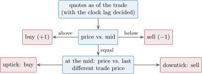
The trade sign is when a trade was initiated by a buyer (an order that took the ask) and when initiated by a seller. The tick rule signs a trade if its price is above the last different trade price and if below. The quote rule signs it if its price is above the prevailing mid and if below. The Lee–Ready algorithm applies the quote rule and falls back on the tick rule for trades at the mid.
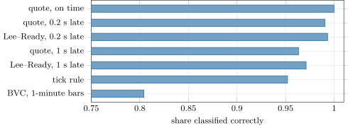
Most public trade data do not say who initiated a trade, and the rules infer it. Lee and Ready (1991) identified the two problems of the quote rule: quotes may be recorded ahead of the trades that triggered them, and trades inside the spread are not readily classifiable. Timing is the practical enemy. On the simulated tape, where every trade happens at the touch, the quote rule with the quotes prevailing at the trade signs 100% of trades correctly; with quotes 0.2 seconds stale, 99.1%; one second stale, 96.3% (Lee–Ready 97.1%); the tick rule, which needs no quotes, 95.2% (Figure 9.2). Real data do worse, since real trades happen inside the spread, in hidden orders and in auctions.
Definition 9.2 (Bulk volume classification)
Bulk volume classification (BVC) splits a bar’s volume into buys and sells without signing individual trades: the buy share is , with the bar’s price change and its standard deviation across bars.
BVC was introduced with VPIN for data too coarse to sign trade by trade. It pays for that: on one-minute bars of the simulated tape it classifies 80.4% of the volume correctly, against 95% or more for the trade-level rules, and Chakrabarty, Pascual and Shkilko found on a large sample of US stocks that the tick rule and Lee–Ready classify significantly better than BVC.
firm.tape, seed 9.9.2 Order-sign autocorrelation
Definition 9.3 (Order-sign autocorrelation, metaorder)
The order-sign autocorrelation is the autocorrelation function of the signs of successive aggressive orders. A metaorder is a large order executed as a sequence of smaller child orders over time.
Order signs are not independent: buys follow buys. Lillo and Farmer (2004) found on the London Stock Exchange that the autocorrelation of order signs decays roughly as a power of the lag with exponent 0.6, a Hurst exponent of 0.7 (Book 4, chapter 17): long memory. The explanation they and Mike later gave is the splitting of metaorders.
Proposition 9.4 (Metaorders make order signs long-memory)
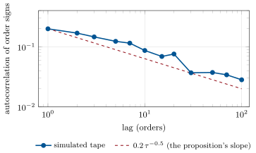
If metaorders are split into child orders of constant size, all of the metaorder’s sign, and the distribution of metaorder sizes has a power-law tail with , the autocorrelation of child-order signs decays asymptotically as , and the Hurst exponent of the sign series is .
Proof. Admitted here. ∎
The result is Lillo, Mike and Farmer’s (2005); the Hurst exponent follows from the decay exponent by .
The simulator’s noise traders draw metaorder lengths from a Pareto law with tail exponent 1.5, so the proposition predicts . The 7 273 aggressive orders of the simulated tape have sign autocorrelations of 0.20 at lag 1, 0.087 at lag 10 and 0.028 at lag 100 (Figure 9.3), and a Hurst exponent by aggregated variance of 0.715. Sign memory is the reason signed volume is a predictor of the next signs, and not only a summary of the past: a buying metaorder that has shown itself will probably keep buying.
How much of that memory is a forecast of prices? The signed-flow imbalance of the last aggressive orders (the first card below) was measured against three targets on the simulated tape: the next order’s sign, the mid-price change over the next ten seconds, and, as a control, the change over the previous ten seconds.
| last orders | corr. with next sign | next sign right | corr. with next 10 s | corr. with last 10 s |
|---|---|---|---|---|
| 5 | 0.25 | 56.1% | 0.16 | 0.22 |
| 20 | 0.24 | 58.4% | 0.14 | 0.31 |
| 100 | 0.18 | 57.1% | 0.12 | 0.17 |
The flow forecasts the next sign well and the next price change less well, and for twenty orders it is twice as correlated with the change that has already happened as with the one to come: much of what the flow knows, the price already shows. Order signs are predictable without prices being so, which is Lillo and Farmer’s point: the liquidity on the other side adjusts.
firm.tape, seed 9.9.3 Flow toxicity
Definition 9.5 (Flow toxicity, VPIN)
Flow toxicity is the adverse selection that order flow imposes on the liquidity providers who trade against it: its aggressors are informed, and the resting side loses on average. VPIN (volume-synchronised probability of informed trading) cuts the trade sequence into buckets of equal volume and, at the end of each bucket, averages over the last buckets, with and the bucket’s buy and sell volume.
VPIN measures one-sided flow. Its authors define toxicity as adverse selection of the market makers (Easley, López de Prado and O’Hara, 2012) and argue that one-sided volume is how it shows. Toxicity itself, though, is directly measurable after the fact: the mark-out of Book 2, chapter 15, of trades against their resting side. The simulated episode separates the two cleanly. During it, the aggressors’ mark-out ten seconds after the trade goes from ticks (they pay the half-spread) to (they win): the flow is toxic by definition. VPIN, over buckets of 2 649 shares and a window of twenty, rises from 0.31 to 0.35, 13%; its maximum over the three hours falls outside the episode, 20 minutes after it ends (Figure 9.4). The informed traders of the simulator buy when the efficient price is above the mid and sell when below, so their flow is not one-sided over a bucket; the noise traders’ metaorders are. One-sided volume and informed volume are different things.
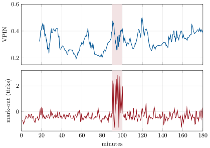
firm.tape, seed 9.The flash-crash debate had the same shape. Easley, López de Prado and O’Hara (2011) found historically high VPIN readings before the crash; Andersen and Bondarenko (2014) found VPIN a poor predictor of short-run volatility. A simulator cannot settle a debate about real markets, but it can show a measure failing on a toxicity it was designed for, which is reason enough to validate it on data where the truth is known before trusting it where it is not. The mark-out measure has its own cost: it needs the future (ten seconds here), so it detects late; in the episode it first crosses its pre-episode 95th percentile 40 seconds after the start, VPIN after 16 seconds, but VPIN also spends 6.0% of the rest of the session above its threshold.
9.4 Fitted excitation intensities
Aggressive orders cluster in time, and a Hawkes process (Book 4, chapter 7) is the standard description: each order raises the intensity of the next. Its branching ratio is the share of orders triggered by earlier ones. On a flat version of the simulated tape (no activity process, no news, no informed traders) the maximum-likelihood fit recovers 0.403, against the 0.4 the simulator plants. On the chapter’s tape the fit gives 0.65. Nothing in the order-generating mechanism changed; what changed is that activity rises and falls for other reasons, and a Hawkes process attributes every cluster to self-excitation. A fitted branching ratio is an upper bound on endogeneity unless the baseline is allowed to vary. As features, the fitted buy and sell intensities and their difference summarise how excited each side of the flow is.
9.5 Large trades and metaorders
Definition 9.6 (Kyle’s lambda)
Kyle’s lambda is the price impact per unit of signed order flow: the slope of price changes on net signed volume over the same intervals, after the parameter of Kyle’s (1985) model of an informed trader and market makers.
On the simulated tape, over ten-second intervals, lambda is 0.10 ticks per 100 shares of net buying, with an of 14%: far below the 53% of order-flow imbalance (chapter 8), because signed trade volume misses the cancellations and additions that move the quotes, as Cont, Kukanov and Stoikov noted for real data. Lambda is a liquidity feature (a stock whose price moves more per share traded is less liquid) and a cost input (chapter 27). Metaorder detection starts from the same flows: a run of same-sign orders of similar size at regular intervals, an unusual share of one side over minutes, a VPIN-like imbalance on a volume clock. The chapter’s memory result says why it works: children of one parent share its sign.
9.6 Predictor cards
Predictor card 9.1 — Signed-flow imbalance
Definition. over the aggressive orders of the last seconds (or last orders), the sign.
Inputs and timestamps. Trades with receive times; signs from the feed’s aggressor flag or from Lee–Ready with quotes as of the trade’s receive time.
Rationale. Order signs have long memory (Proposition 9.4); metaorders continue.
Horizon and half-life. The next orders; sign autocorrelation 0.20 at one order, 0.087 at ten on the simulated tape; over twenty orders it gets the next sign right 58.4% of the time.
Normalisation. By total volume; across instruments by average trade size.
Failure modes. Misclassification with stale quotes; the price moves before the flow is seen (the impact is already in the price).
Sources. Lillo and Farmer (2004); Lillo, Mike and Farmer (2005); rs_tradeflow.memory.
Predictor card 9.2 — VPIN
Definition. Mean absolute buy–sell imbalance over the last volume buckets, divided by the bucket size.
Inputs and timestamps. Trades, signed (or BVC on bars), cut into equal-volume buckets.
Rationale. Toxic flow is one-sided (Easley, López de Prado and O’Hara, 2012).
Horizon and half-life. Minutes to hours. On the simulated episode it rises 13% while the aggressors’ mark-out turns from to ticks.
Normalisation. Bounded in ; its level depends on the bucket size and window.
Failure modes. Informed flow that is not one-sided; one-sided flow that is not informed (metaorders, index rebalancing); poor volatility prediction (Andersen and Bondarenko, 2014).
Sources. As cited; rs_tradeflow.toxicity_race.
9.7 Tutorial: signing and weighing the flow
Goal. Sign the simulated tape’s trades by every rule, measure the memory of order signs and fit a Hawkes process, and race VPIN against the mark-out through the toxic episode. End state: Figures 9.2, 9.3 and 9.4; the Hawkes branching ratios 0.65 and 0.403.
The signing rules. The tick rule carries the last price change forward; Lee–Ready uses the quote rule and the tick rule for trades at the mid.
def tick_rule(price) -> np.ndarray:
    p = np.asarray(price, float)
    out = np.zeros(len(p), int)
    last = 0
    for i in range(1, len(p)):
        if p[i] > p[i - 1]:
            last = 1
        elif p[i] < p[i - 1]:
            last = -1
        out[i] = last
    return out


def quote_rule(price, bid, ask, tol: float = 1e-9) -> np.ndarray:
    mid = 0.5 * (np.asarray(bid, float) + np.asarray(ask, float))
    d = np.asarray(price, float) - mid
    return np.where(np.abs(d) < tol, 0, np.sign(d)).astype(int)


def lee_ready(price, bid, ask) -> np.ndarray:
    q = quote_rule(price, bid, ask)
    t = tick_rule(price)
    return np.where(q != 0, q, t)
Listing 9.1. Tick rule, quote rule and Lee–Ready. code/firm/tradeflow/firm_tradeflow.py VPIN. Trades are poured into buckets of equal volume, split where a trade straddles two buckets.
def vpin(buy_volume, volume, bucket: float, n: int) -> np.ndarray:
    """Cut the trade sequence into buckets of `bucket` shares (a trade may be split between buckets); VPIN at the end
    of each bucket is sum over the last n buckets of |V_buy - V_sell| / (n * bucket). buy_volume is the buy part of
    each trade's volume (the size itself for a buy, 0 for a sell, or a fraction of it under BVC)."""
    bv, v = np.asarray(buy_volume, float), np.asarray(volume, float)
    imb, fill, buys = [], 0.0, 0.0
    for b_i, v_i in zip(bv, v, strict=True):
        frac_b = b_i / v_i if v_i > 0 else 0.0
        left = v_i
        while left > 0:
            take = min(left, bucket - fill)
            fill += take
            buys += take * frac_b
            left -= take
            if fill >= bucket - 1e-9:
                imb.append(abs(2.0 * buys - bucket))
                fill, buys = 0.0, 0.0
    imb = np.array(imb)
    out = np.full(len(imb), np.nan)
    if len(imb) >= n:
        cs = np.cumsum(imb)
        out[n - 1:] = (cs[n - 1:] - np.r_[0.0, cs[:-n]]) / (n * bucket)
    return out
Listing 9.2. VPIN on volume buckets. code/firm/tradeflow/firm_tradeflow.py - Run
signing(),memory(),signed_flow(),hawkes_fits(),toxicity_race(),kyle()andfig_tradeflow.py.
What to change next. Make the informed traders one-sided (buy only while the episode lasts) and see VPIN respond; fit a Hawkes process with a baseline that follows the activity level and watch the branching ratio fall back.
9.8 Build: the trade-flow toolkit
Purpose. Signing, memory, toxicity and impact measures on the miniature firm’s trade data, for features (Books 8, 11, 12) and for execution research (Book 10).
Interface. tick_rule, quote_rule, lee_ready, bvc, sign_acf, hurst_aggvar, vpin(buy_volume, volume, bucket, n), kyle_lambda, markout_toxicity, aggregate_orders.
Rules. Quotes passed in are those prevailing at each trade’s knowledge time; a trade that straddles a volume bucket is split proportionally; executions of one aggressive order are aggregated before sign statistics.
Acceptance tests. code/firm/tradeflow/tests/: the three rules on a hand-built sequence and BVC’s symmetry; VPIN of a balanced and of a one-sided sequence; for independent data and a sign autocorrelation that vanishes beyond a run’s length; a known lambda recovered; order aggregation.
Stretch. Hawkes fits with a time-varying baseline; metaorder detection by change points in signed flow; mark-outs by counterparty type.
Sources and further reading
- C. M. C. Lee and M. J. Ready, “Inferring trade direction from intraday data”, Journal of Finance 46(2), 1991.
- B. Chakrabarty, R. Pascual and A. Shkilko, “Evaluating trade classification algorithms: bulk volume classification versus the tick rule and the Lee–Ready algorithm”, Journal of Financial Markets 25, 2015.
- F. Lillo and J. D. Farmer, “The long memory of the efficient market”, Studies in Nonlinear Dynamics and Econometrics 8(3), 2004; F. Lillo, S. Mike and J. D. Farmer, “Theory for long memory in supply and demand”, Physical Review E 71, 2005.
- D. Easley, M. López de Prado and M. O’Hara, “The microstructure of the ‘flash crash”’, Journal of Portfolio Management 37(2), 2011; “Flow toxicity and liquidity in a high-frequency world”, Review of Financial Studies 25(5), 2012.
- T. G. Andersen and O. Bondarenko, “VPIN and the flash crash”, Journal of Financial Markets 17, 2014.
- A. S. Kyle, “Continuous auctions and insider trading”, Econometrica 53(6), 1985.
9.9 Exercises
Exercise 9.1 ★
Trades at 20.00, 20.01, 20.01, 20.00, 19.99 with the quotes 20.00–20.01 throughout. Sign each by the tick rule and by Lee–Ready.
Solution
Solution of Exercise 9.1.
The mid is 20.005. Tick rule: unclassified (no earlier price), , (a zero tick keeps the last sign), , . Lee–Ready: every trade is off the mid, so it is the quote rule: , , , , . The two differ on the first trade only.
Exercise 9.2 ★
A one-minute bar’s price change is standard deviations. What share of its volume does BVC classify as buys?
Solution
Solution of Exercise 9.2.
: 78.8% of the bar’s volume is classified as buys, whatever the trades inside it actually were.
Exercise 9.3 ★
Metaorders with a size tail exponent of 1.4: what decay exponent and Hurst exponent does Proposition 9.4 predict?
Solution
Solution of Exercise 9.3.
Decay exponent ; Hurst exponent .
Exercise 9.4 ★★
Five volume buckets of 1 000 shares have buy volumes 700, 400, 900, 500 and 200. What is VPIN over the last five buckets?
Solution
Solution of Exercise 9.4.
The imbalances are 400, 200, 800, 0 and 600, summing to 2 000; VPIN .
Exercise 9.5 ★★
Kyle’s lambda is 0.10 ticks per 100 shares. What price move does a net purchase of 3 000 shares over ten seconds imply, and why is the estimate noisier than one based on OFI?
Solution
Solution of Exercise 9.5.
ticks. Signed trade volume sees only the executions; the quotes also move when orders are cancelled or added, which OFI counts and signed volume does not. On the simulated tape the is 14% against OFI’s 53%, so the slope is estimated from a relation that leaves most of the price change unexplained.
Exercise 9.6 ★★
Why does a Hawkes fit on data whose baseline activity varies overstate the branching ratio? Give the intuition with two regimes of different constant intensity.
Solution
Solution of Exercise 9.6.
Take a Poisson process with intensity for half the time and for the other half, each regime long. No event causes another, but an event is more likely to fall in the busy regime, and then more events follow it soon: counts are over-dispersed compared with one Poisson process. A Hawkes process with a constant baseline has only one way to produce that clustering, excitation, so the fit puts mass in the kernel, and the more the regimes differ the higher the branching ratio. On the chapter’s tape the fit gives 0.65 against the 0.4 planted, which the flat tape recovers (0.403).
Exercise 9.7 ★★★
Coding. With the chapter’s tape, compute the share of trades signed correctly by the quote rule with quotes 0.05, 0.5 and 2 seconds late. How fast does accuracy fall with staleness?
Solution
Solution of Exercise 9.7.
rs_tradeflow.stale_quotes: 99.7% with quotes 0.05 seconds late, 97.9% at 0.5 seconds and 93.8% at 2 seconds. The loss is about five points per second of staleness at first and slows (6.2 points at two seconds): the older the quote, the more likely the mid has moved past the trade price, but a quote that has moved once may move back.
Exercise 9.8 ★★★
Find the flaw. “VPIN reached its highest level of the year an hour before the crash, so VPIN predicts crashes.”
Solution
Solution of Exercise 9.8.
It is a statement chosen after the event. A warning is useful only with its false-alarm rate: how often VPIN reached such levels with no crash, and whether high readings were followed by high volatility on average (Andersen and Bondarenko found they were a poor predictor of it). A highest reading of the year is also one draw among the year’s hours; some hour before any event is the maximum of its neighbourhood. And the level depends on choices (bucket size, window, the signing method) that must be fixed before the event for the claim to count.
9.10 Problem: Did VPIN See It Coming?
Problem 9.1
Weekend problem — a toxicity measure against the truth
The chapter’s tape: three hours, a ten-minute episode from minute 90 in which the efficient price moves eight times faster and noise trading does not rise, seed 9.
Part I — The truth.
- What share of the flow is informed before and during the episode?
- What is the aggressors’ ten-second mark-out, in ticks, before and during?
- Why is the mark-out negative before the episode?
- Is the episode’s flow toxic by the definition of the chapter?
Part II — VPIN.
- What bucket size and window does the chapter use, and how many buckets does the session have?
- What are VPIN’s mean before and during the episode?
- When does VPIN reach its maximum?
- When does it first cross its pre-episode 95th percentile after the episode starts, and what share of the rest of the session is above that threshold?
- Why does VPIN barely move?
Part III — The mark-out measure.
- What are its mean before and during, and when does it peak?
- When does it first cross its threshold, and why is it later than VPIN?
- What share of the rest of the session is above its threshold?
- Which measure would you use to protect a market maker, and which to study toxicity after the fact?
Part IV — Beyond.
- What would make informed flow one-sided, and VPIN useful?
- What does the Hawkes fit give on this tape and on the flat tape?
- What are Kyle’s lambda and its at ten seconds?
- Which of the chapter’s features could detect the episode fastest, and at what cost in false alarms?
- State the named result: VPIN’s rise during an episode in which the informed share triples and the aggressors’ mark-out turns from to ticks.
- What does the result say about validating a toxicity measure?
- In one sentence: what is toxic flow?
Solution
Solution of Problem 9.1.
- 15% before the episode, 45% during it: the informed share nearly triples.
- ticks before, during (the mid ten seconds after the trade, minus the trade price, in the direction of the trade).
- Aggressors pay the half-spread, half a tick, and most of them are noise traders whose orders carry no information: the resting side earns the spread.
- Yes: the aggressors win and the liquidity providers lose on average, the definition of toxic flow.
- Buckets of 2 649 shares, of the session’s volume, so 400 buckets, and a window of 20 buckets.
- 0.31 before, 0.35 during: a rise of 13%.
- At minute 119.7, 20 minutes after the episode ends.
- 16 seconds after the episode starts; VPIN is above the same threshold for 6.0% of the session outside the episode.
- The informed traders buy when the efficient price is above the mid and sell when it is below; as that price wanders both ways, their flow over a bucket (27 seconds on average) is not one-sided. The one-sided runs come from the noise traders’ metaorders, which the episode replaces with informed flow rather than adds to.
- before, during; it peaks at 5 740 seconds, inside the episode.
- At 5 440 seconds, 40 seconds after the start: each value waits ten seconds for its mark-out, and the rolling one-minute mean needs toxic trades to fill it.
- 8.4%.
- For studying toxicity after the fact, the mark-out: it is toxicity by definition. To protect a market maker in real time, the mark-outs of its own recent fills at a short horizon together with the order-book features of chapter 8; VPIN has not shown here that it would help.
- Informed traders with a signal that points one way for longer than a bucket, a single large informed order split over minutes, or news that moves the value in one step. VPIN measures that case, not this one.
- 0.65 on this tape; 0.403 on the flat tape, against the planted 0.4.
- 0.10 ticks per 100 shares of net buying, with an of 14%.
- VPIN crosses its threshold first, 16 seconds in, at 6.0% false alarms; the mark-out 40 seconds in, at 8.4%. Neither is clean, and VPIN’s early crossing is not matched by a rise in its level.
- Named result. When the informed share of the flow goes from 15% to 45% and the aggressors’ mark-out turns from to ticks, VPIN rises only 13%, from 0.31 to 0.35, and reaches its maximum 20 minutes after the episode ends.
- A toxicity measure must be tested against toxicity itself (the mark-outs), on data where it is known, before it is trusted where it is not; a plausible story linking the measure to informed trading is not a test.
- Toxic flow is order flow whose aggressors are informed, so that the liquidity providers who trade against it lose on average.
9.11 Interview questions
Interview question 9.1 ★ researcher, trader
How would you decide whether a trade was a buy or a sell if the data do not say?
Solution
Solution of Interview question 9.1.
With quotes, compare the trade price with the prevailing mid, taking the quotes as of the trade’s timestamp and checking how the two clocks align (Lee and Ready, 1991); fall back on the tick rule at the mid. Without quotes, the tick rule. Measure the error where the truth is known (a feed with an aggressor flag, or a simulator): on the chapter’s tape a quote one second stale loses 3.7 points of accuracy.
Interview question 9.2 ★★ researcher
Why are the signs of market orders autocorrelated, and why does that not make prices predictable in the same way?
Solution
Solution of Interview question 9.2.
Metaorders are split into many child orders of one sign, so signs persist (Lillo, Mike and Farmer, 2005). Prices stay close to unpredictable because liquidity adjusts: as a run of buys continues, the impact of each further buy falls, and sellers refill the ask, so the predictable sign does not become a predictable price move of the same size.
Interview question 9.3 ★★ trader, researcher
What is flow toxicity, and how would you measure it for your own market-making book?
Solution
Solution of Interview question 9.3.
Flow is toxic when those who trade against it lose on average. Measure it by mark-outs: for each of the book’s fills, the mid a few horizons later minus the fill price, from the book’s side, by client, venue, time of day and size; a mark-out that turns negative quickly is toxic flow.
Interview question 9.4 ★★ researcher, mle
You fit a Hawkes process to trade times and get a branching ratio of 0.9. What else could explain it?
Solution
Solution of Interview question 9.4.
A baseline that varies (time of day, news, volatility regimes) produces clusters that a constant-baseline fit attributes to excitation. Fit with a baseline that follows the time of day or a measured activity level, compare on held-out data, and check on simulated data with a known branching ratio: the chapter’s tape gives 0.65, its flat version 0.403 against 0.4.
Interview question 9.5 ★★ researcher
Explain VPIN and its main criticism.
Solution
Solution of Interview question 9.5.
Cut trades into equal-volume buckets, sign them (or classify bars by BVC), and average the absolute buy–sell imbalance over the last buckets, divided by the bucket size; the claim is that one-sided flow is toxic. The criticism: it was a poor predictor of short-run volatility (Andersen and Bondarenko, 2014), its level depends on arbitrary choices, and one-sided flow need not be informed, nor informed flow one-sided.
Interview question 9.6 ★★★ researcher
Derive the relation between the tail exponent of metaorder sizes and the Hurst exponent of order signs, and test it on a series.
Solution
Solution of Interview question 9.6.
If metaorder sizes have tail exponent , the sign autocorrelation decays as (Lillo, Mike and Farmer, 2005), and a series whose autocorrelation decays as with has partial sums with variance growing like , so . Test: aggregate the executions into orders, compute the variance of block sums of signs across scales and regress in logs. The chapter’s tape, with , predicts 0.75 and gives 0.715.