Research Craft: Predictors, Backtests, Measurement, Portfolios · Research
26Portfolio Construction II
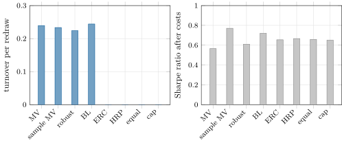
Move one stock’s alpha by a basis point and a long-only mean–variance book of fifty names moves by 0.03 per cent of its capital on average, 0.33 per cent at worst. Draw the forecast’s noise again (an equally good forecast, with different errors) and the book turns over 24 per cent. Over eight years its information about the stocks does not show: after costs, its Sharpe ratio of 0.57 is within one standard error of holding the market. Over days rather than months the picture reverses: how a book moves matters more than where it points. With three true signals that decay at different speeds and trading costs that grow with the square of the trade, re-optimising every day to the mean–variance portfolio nets a Sharpe ratio of ; trading part of the way each day towards Gârleanu and Pedersen’s aim portfolio nets 4.06. This chapter builds firm.allocation: robust optimisation, Black–Litterman, risk parity in two forms, and the aim portfolio.
26.1 Robust optimisation
Definition 26.1 (Robust portfolio optimisation, uncertainty set)
Robust portfolio optimisation maximises the worst case of the objective over an uncertainty set of inputs. For an ellipsoid of alphas the worst-case expected return is , and the problem is a second-order cone programme (Goldfarb and Iyengar).
The penalty grows with the size of the book along the directions in which the alpha is least certain, which are the directions the error maximiser of chapter 25 loved. The chapter’s solver (robust_mv) needs no cone solver; it works by majorisation: since with equality at , each step solves a quadratic programme with the square root replaced by a quadratic that touches it at the current book, and the objective rises at every step (Listing 26.1).
The chapter’s first book holds the fifty largest names of chapter 25’s universe, long only, fully invested, at most 10% a name, rebuilt at the 95 month-ends with chapter 25’s alpha and chapter 24’s risk model (). The robust version uses an ellipsoid of three standard errors of the alpha across names. A basis point added to one stock’s alpha moves the plain mean–variance book by 0.029% of capital on average and 0.33% at most; the robust book by 0.028% on average and 0.12% at most. Robustness does not change how much a book listens to its forecast on average; it removes the largest jumps, which happen where two names are nearly interchangeable to the optimiser.
26.2 Views blended with equilibrium
Definition 26.2 (Implied equilibrium returns, Black–Litterman model)
The implied equilibrium returns of a market portfolio are : the expected returns for which is the mean–variance optimum. The Black–Litterman model (Black and Litterman, 1992) treats as a prior with covariance and views with uncertainty as observations, and optimises on the posterior mean with covariance .
Black–Litterman changes the question from “what are the expected returns?” to “how far from the market should the forecast move me?” Without views the optimal book is the market; with a view held with certainty the posterior meets it exactly; the book in between is a blend. The chapter’s version takes capitalisation weights as , each stock’s alpha as a view on its return in excess of , (the usual default) and view uncertainties equal to times each stock’s variance. Its sensitivity to one basis point is 0.031% on average and 0.11% at most, and its book stays near the market’s: its realised volatility is 19.6%, the market’s 19.5%, where mean–variance’s is 15.8%.
26.3 Risk parity and risk budgeting
Definition 26.3 (Risk contribution, risk budgeting, equal risk contribution portfolio, risk parity)
The risk contribution of position is , its Euler share of the variance (Book 6, chapter 20); the shares sum to one. Risk budgeting chooses long-only weights whose risk contributions equal given budgets; the equal risk contribution portfolio gives every position the same share (Maillard, Roncalli and Teïletche). Risk parity is the practice of allocating across asset classes by equal risk contributions, usually with leverage.
Proposition 26.4 (Risk budgets by Newton’s method)
The function is strictly convex on and its minimiser satisfies ; the weights therefore have risk contributions .
Proof. The Hessian is positive definite, and at the boundary and at infinity, so there is one minimiser, where componentwise. Risk contributions are invariant to scaling , and . ∎
Risk-based books ignore the alpha, so they do not move when it does: their sensitivity is zero, by construction and without merit. Their virtue is elsewhere. Maillard, Roncalli and Teïletche showed that the equal risk contribution portfolio’s volatility lies between the minimum-variance and the equally weighted portfolios’, and so it does here: 18.4% against 19.3% for equal weights. Asness, Frazzini and Pedersen explained why risk parity across asset classes has earned more than its risk suggests: investors averse to leverage bid up risky assets, leaving safer ones with higher risk-adjusted returns for anyone who can lever them.
26.4 Hierarchical allocation
Definition 26.5 (Hierarchical risk parity)
Hierarchical risk parity (López de Prado) orders the assets by single-linkage clustering of correlation distances , and splits the capital recursively: each block of the ordered list is cut in two, and the halves receive capital in inverse proportion to the variance of their inverse-variance portfolios.
Hierarchical risk parity never inverts the covariance matrix, so it cannot amplify its smallest eigenvalues; on a diagonal covariance it gives the inverse-variance weights, and on a matrix of blocks it splits the capital between the blocks before it looks inside them. On the fifty names it holds at most 5.8% of capital in one stock and realises 17.8% volatility. The comparison of the eight rules over 95 months, after costs of ten basis points a trade:
| rule | redraw turnover | Sharpe | after costs | volatility | turnover |
|---|---|---|---|---|---|
| mean–variance, factor model | 23.9% | 0.62 | 0.57 | 15.8% | 33% |
| mean–variance, sample covariance | 23.4% | 0.82 | 0.77 | 15.9% | 31% |
| robust mean–variance | 22.4% | 0.66 | 0.61 | 15.8% | 31% |
| Black–Litterman | 24.4% | 0.75 | 0.72 | 19.6% | 27% |
| equal risk contribution | 0 | 0.66 | 0.65 | 18.4% | 7% |
| hierarchical risk parity | 0 | 0.69 | 0.67 | 17.8% | 14% |
| equal weights | 0 | 0.67 | 0.66 | 19.3% | 5% |
| capitalisation weights | 0 | 0.66 | 0.65 | 19.5% | 6% |
The redraw turnover is the one-way turnover when the forecast’s noise is drawn again; the last column is the monthly one-way turnover. A Sharpe ratio measured over 7.9 years has a standard error of about 0.4, and every row is within it of every other. The long-only books are dominated by the market they hold; their alphas are a small tilt, and the forecast’s noise, redrawn, moves the alpha-based books by a quarter of their capital. That is the honest conclusion of a comparison that is often presented as a contest: the rules differ in stability, concentration and cost, not detectably in performance.
rs_allocation.26.5 Multi-period optimisation with costs
Definition 26.6 (Aim portfolio, multi-period optimisation)
Multi-period optimisation chooses trades by planning a sequence of future books under forecasts of returns, risks and costs, and executes the first (Boyd and co-authors). With quadratic costs and signals whose predictive power decays at rates , Gârleanu and Pedersen show that the optimal book trades each period a fraction of the way from the current book to the aim portfolio , which weights slow signals more than fast ones, with the positive root of and the discount rate.
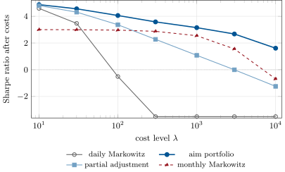
The chapter’s second book holds the same fifty names long and short, daily, with the simulation’s three planted expected-return components as signals: the persistent drift (half-life 504 days, a day), the post-earnings drift (sixty days, ) and the one-day reversal (). They are the true expected returns, so gross Sharpe ratios are high; the question is only what trading them costs. puts the daily Markowitz book at 10% annual volatility. Four rules, at a cost level :
| rule, | Sharpe ratio | after costs | costs a year | daily turnover |
|---|---|---|---|---|
| re-optimise daily to Markowitz | 5.14 | 56.6% | 2.11 | |
| aim portfolio (trade 0.56 of the gap) | 4.74 | 4.06 | 4.0% | 0.56 |
| partial adjustment to Markowitz (0.56) | 5.07 | 3.36 | 12.6% | |
| rebalance monthly to the slow signals | 3.01 | 2.96 | 0.2% |
The daily Markowitz book chases the reversal, the largest and shortest of the three signals, and pays for it every day. Partial adjustment trades less but still aims at the reversal. The aim portfolio aims mostly at the slow signals: with , the reversal enters with weight , the post-earnings drift with 0.987 and the persistent drift with 0.999, and the book moves 56% of the way each day. At ten times the cost () the aim rule trades 0.23 of the gap and still nets 3.15; daily re-optimisation nets with costs of 566% a year, partial adjustment 1.08, the monthly rebalance 2.55. At only the aim rule survives, at 1.61 (Figure 26.2).
rs_allocation.multiperiod.26.6 Tutorial: the one-basis-point flip
Goal. Build the fifty-name book by eight rules, measure their stability and realised performance, then trade the three planted signals daily under four rules and a range of costs. End state: the two tables, Figures 26.1 and 26.2.
Robust mean–variance by majorisation.
def robust_mv(alpha, Sigma, Omega, kappa: float, gamma: float, lo=0.0, hi=1.0, budget=1.0, iters: int = 50):
    """sqrt(x) <= x / (2 s) + s / 2 with equality at x = s^2: each step maximises the minorant alpha'w -
    kappa w'Omega w / (2 s) - gamma/2 w'Sigma w, s = sqrt(w_prev' Omega w_prev); the objective rises monotonically."""
    alpha, Sigma, Omega = (np.asarray(a, float) for a in (alpha, Sigma, Omega))
    w = mean_variance(alpha, Sigma, gamma, lo, hi, budget)
    for _ in range(iters):
        s = max(math.sqrt(float(w @ Omega @ w)), 1e-12)
        new = _box_qp(gamma * Sigma + kappa / s * Omega, -alpha, lo, hi, budget)
        if np.abs(new - w).max() < 1e-10:
            return new
        w = new
    return w
Listing 26.1. A sequence of quadratic programmes for the robust objective. code/firm/allocation/firm_allocation.py Risk budgets by Newton’s method.
def risk_budget(Sigma, b, tol: float = 1e-12, max_iter: int = 100):
    """Minimise y'Sigma y / 2 - sum b_i log y_i (strictly convex on y > 0) by Newton's method with backtracking;
    at the optimum y_i (Sigma y)_i = b_i, so w = y / sum y has risk contributions b."""
    S, b = np.asarray(Sigma, float), np.asarray(b, float)
    y = b / np.sqrt(np.diag(S))
    f = lambda v: 0.5 * v @ S @ v - b @ np.log(v)  # noqa: E731
    for _ in range(max_iter):
        g = S @ y - b / y
        H = S + np.diag(b / y**2)
        d = -np.linalg.solve(H, g)
        if -g @ d < tol:
            break
        t = 1.0
        while np.any(y + t * d <= 0) or f(y + t * d) > f(y) + 0.25 * t * (g @ d):
            t *= 0.5
        y = y + t * d
    return y / y.sum()
Listing 26.2. Weights with given risk contributions. code/firm/allocation/firm_allocation.py The aim portfolio and the trade rate.
def gp_trade_rate(gamma: float, lam: float, rho: float) -> float:
    """Garleanu-Pedersen: a solves a^2 (1-rho) + a (gamma (1-rho) + lam rho) - gamma lam (1-rho) = 0 (costs
    lam/2 dx'Sigma dx, risk gamma/2 x'Sigma x, discount 1 - rho); the book trades a/lam of the gap each period."""
    c = gamma * (1 - rho) + lam * rho
    a = (-c + math.sqrt(c * c + 4 * gamma * lam * (1 - rho) ** 2)) / (2 * (1 - rho))
    return a / lam


def gp_aim(Sigma, signals, phis, gamma: float, a: float):
    """The aim portfolio: the Markowitz portfolio of each signal's expected return, down-weighted by 1 + phi a /
    gamma for a signal whose predictive power decays at rate phi per period (signals: list of (n,) expected-return
    contributions, i.e. B_k f_k)."""
    total = sum(np.asarray(s, float) / (1 + phi * a / gamma) for s, phi in zip(signals, phis, strict=True))
    return np.linalg.solve(gamma * np.asarray(Sigma, float), total)
Listing 26.3. Gârleanu and Pedersen’s rule. code/firm/allocation/firm_allocation.py - Run
rs_allocation.stability,redraw_turnover,backtestfor each rule,multiperiodfor each rule and cost, andfig_allocation.py.
What to change next. Replace the true signals by noisy forecasts and see the aim rule’s advantage grow (it averages the noise, as chapter 25’s turnover limit did); give the equal-risk-contribution book leverage to the mean–variance book’s volatility and compare.
26.7 Build: the allocation toolkit
Purpose. The alternatives to plain mean–variance that the firm uses, each with a test of its defining property, and a trading rule for signals of different speeds.
Interface. mean_variance(alpha, Sigma, gamma, lo, hi, budget), robust_mv(alpha, Sigma, Omega, kappa, gamma, lo, hi, budget), implied_returns(Sigma, w_mkt, gamma), black_litterman(pi, Sigma, P, q, Omega, tau), risk_contributions(w, Sigma), risk_budget(Sigma, b), erc(Sigma), hrp(Sigma), gp_trade_rate(gamma, lam, rho), gp_aim(Sigma, signals, phis, gamma, a).
Rules. Every rule is judged on stability to a redrawn forecast and on cost-adjusted performance with its standard error; a signal’s decay rate is estimated (chapter 13) before it is traded; fast signals are traded only through a rule that knows they are fast.
Acceptance tests. code/firm/allocation/tests/: mean–variance against its closed form; the robust objective above the plain book’s, and equal to it at ; implied returns reproducing the market; a certain view met and a worthless one ignored; risk contributions equal to their budgets; HRP equal to inverse variance on a diagonal matrix and splitting blocks evenly; the trade rate’s limits and the aim’s down-weighting.
Stretch. The aim rule with linear costs (no-trade regions); robust optimisation over the covariance too; hierarchical risk budgets.
Sources and further reading
- F. Black and R. Litterman, “Global portfolio optimization”, Financial Analysts Journal 48(5), 1992; PyPortfolioOpt,
black_litterman(documented implementation, after He and Litterman). - D. Goldfarb and G. Iyengar, “Robust portfolio selection problems”, Mathematics of Operations Research 28(1), 2003.
- S. Maillard, T. Roncalli and J. Teïletche, “The properties of equally weighted risk contribution portfolios”, Journal of Portfolio Management 36(4), 2010.
- M. López de Prado, “Building diversified portfolios that outperform out of sample”, Journal of Portfolio Management 42(4), 2016.
- N. Gârleanu and L. H. Pedersen, “Dynamic trading with predictable returns and transaction costs”, Journal of Finance 68(6), 2013.
- S. Boyd et al., “Multi-period trading via convex optimization”, Foundations and Trends in Optimization 3(1), 2017.
- C. S. Asness, A. Frazzini and L. H. Pedersen, “Leverage aversion and risk parity”, Financial Analysts Journal 68(1), 2012.
26.8 Exercises
Exercise 26.1 ★
Two uncorrelated assets have volatilities of 20% and 10%. Give the equal-weight portfolio’s volatility, and the weights of the equal risk contribution portfolio.
Solution
Solution of Exercise 26.1.
. With no correlation the equal risk contributions are equal after normalisation, so : and .
Exercise 26.2 ★
Show that with no views the Black–Litterman book is the market portfolio.
Solution
Solution of Exercise 26.2.
Without views the posterior mean is , and the mean–variance optimum on it (with covariance ) is ; with the posterior covariance it is , the market scaled.
Exercise 26.3 ★
With , give the aim portfolio’s weights on signals decaying at , and a day.
Solution
Solution of Exercise 26.3.
: 0.56 for the reversal, 0.987 for the post-earnings drift, 0.999 for the persistent drift.
Exercise 26.4 ★★
Why does robust optimisation cut the largest response to a one-basis-point change but not the average one?
Solution
Solution of Exercise 26.4.
The average response is set by the inverse covariance and , which the robust term changes little. The largest responses come from names the optimiser finds nearly interchangeable, where a small alpha change moves weight from one to the other; the penalty on makes concentrating in either costly, so the book holds both and the flip is damped (0.33% to 0.12% at most).
Exercise 26.5 ★★
Why is the equal risk contribution portfolio’s volatility between the minimum-variance and the equally weighted portfolios’?
Solution
Solution of Exercise 26.5.
It minimises variance subject to a constraint on the diversity of weights ( above a bound): with no constraint the solution is minimum variance, with an infinitely tight one it is equal weights, and the equal risk contribution portfolio is one point on that path (Maillard, Roncalli and Teïletche).
Exercise 26.6 ★★
Why does partial adjustment to the Markowitz portfolio do worse after costs than the aim rule trading at the same rate?
Solution
Solution of Exercise 26.6.
Both trade 56% of the gap each day, but partial adjustment aims at the Markowitz portfolio, dominated by the reversal that decays in a day: it keeps paying to move towards a target that will have moved. The aim portfolio weights the reversal by 0.56 and the slow signals by nearly one, so the target itself moves less.
Exercise 26.7 ★★★
Coding. Run rs_allocation.multiperiod for the four rules at and , and explain which rule survives and why.
Solution
Solution of Exercise 26.7.
At : daily Markowitz , aim 3.15, partial 1.08, monthly 2.55. At : the aim rule 1.61, the monthly rebalance , the others below. The aim rule survives because it adjusts both its target (towards slow signals) and its speed (0.23 of the gap at ) to the costs.
Exercise 26.8 ★★★
Find the flaw. “Hierarchical risk parity beat mean–variance by 0.10 of Sharpe ratio after costs over eight years, so we will switch.”
Solution
Solution of Exercise 26.8.
The difference (0.67 against 0.57) is a quarter of the standard error of a Sharpe ratio over 7.9 years (about 0.4). Switch for reasons that are measured precisely (stability, concentration, turnover), not on this comparison.
26.9 Problem: The One-Basis-Point Flip
Problem 26.1
Weekend problem — stable books and good trades
The chapter’s fifty-name books and daily multi-period rules.
Part I — Stability.
- How much does a basis point on one alpha move each alpha-based book, on average and at most?
- How much does a redrawn forecast move them?
- Why do the risk-based books not move, and why is that no merit?
- What does the robust ellipsoid remove, and what not?
Part II — Equilibrium and risk.
- Write the Black–Litterman posterior mean and explain .
- What are the equal risk contribution and HRP books’ volatilities and largest weights?
- How does HRP avoid inverting the covariance matrix?
- Why can risk parity across asset classes earn more than its risk suggests?
Part III — Performance.
- Give the eight rules’ Sharpe ratios after costs and their standard error.
- What can and cannot be concluded from the comparison?
Part IV — Trading through time.
- What are the three signals and their decay rates?
- Why does daily re-optimisation lose after costs?
- What does the aim portfolio weight, and how fast does it trade at ?
- State the named result: turnover per basis point of alpha perturbation for each method, and the net Sharpe ratio of the aim portfolio against daily re-optimisation.
- How do the rules behave as costs grow tenfold and a hundredfold?
- Why does the monthly rebalance do well at low costs and badly at high ones?
- What would noisy forecasts change?
- Which of the chapter’s rules would you run for a daily signal book?
- How would you estimate ?
- In one sentence: what matters more at a daily horizon, the book or the path to it?
Solution
Solution of Problem 26.1.
- Mean–variance 0.029% and 0.33%; sample covariance 0.028% and 0.24%; robust 0.028% and 0.12%; Black–Litterman 0.031% and 0.11%.
- 23.9%, 23.4%, 22.4% and 24.4% of capital, one way.
- They ignore the alpha; they cannot use it either.
- The largest jumps between near-interchangeable names; not the average response to the forecast.
- ; scales the prior’s uncertainty relative to the views’.
- 18.4% and 17.8% volatility; HRP holds at most 5.8% in a name.
- It orders the assets by clustering and splits capital by inverse variances of sub-blocks, never inverting the matrix.
- Leverage-averse investors overpay for risky assets, leaving safer ones with higher risk-adjusted returns for investors who can lever (Asness, Frazzini and Pedersen).
- 0.57, 0.77, 0.61, 0.72, 0.65, 0.67, 0.66, 0.65; standard error about 0.4.
- Stability, concentration and costs differ; performance differences are not detectable.
- The persistent drift ( a day), the post-earnings drift (1/60), the one-day reversal (1).
- It chases the reversal each day, turning over 2.11 times capital a day at a cost of 56.6% a year.
- The slow signals at nearly full weight, the reversal at 0.56; it trades 0.56 of the gap a day.
- Named result. Per basis point: 0.029% (mean–variance), 0.028% (sample and robust), 0.031% (Black–Litterman), 0 for the risk-based rules; at the aim portfolio nets a Sharpe ratio of 4.06 against for daily re-optimisation.
- At the aim rule nets 3.15, the others 2.55 and below; at only the aim rule is positive (1.61).
- It trades rarely, which is cheap when costs are low, but each monthly jump is large, and quadratic costs punish large trades.
- Noise that is new each day is a fast signal: the aim rule would down-weight it and gain relative to the others.
- The aim rule, with decay rates estimated per signal and estimated from the firm’s own fills.
- From the price impact of the firm’s trades (chapter 27): regress cost on trade size relative to volume and volatility.
- The path: with costs, how a book moves decides more of its net performance than which book it moves to.
26.10 Interview questions
Interview question 26.1 ★ researcher
What problem does Black–Litterman solve, and how?
Solution
Solution of Interview question 26.1.
Mean–variance on raw forecasts gives extreme, unstable books. Black–Litterman starts from the returns that make the market optimal and moves away only as far as views, weighted by their confidence, justify: a Bayesian posterior, whose optimum is the market plus tilts.
Interview question 26.2 ★★ researcher, risk
Explain risk parity. What does it assume, and what does it need to deliver equity-like returns?
Solution
Solution of Interview question 26.2.
Allocate so that each asset class contributes equally to risk, ignoring expected returns (assumed roughly proportional to risk). To reach equity-like returns the low-risk classes, mostly bonds, must be levered; the argument for it is that leverage-averse investors leave safer assets with higher risk-adjusted returns.
Interview question 26.3 ★★ researcher
How does robust optimisation change a mean–variance portfolio? How would you choose the size of the uncertainty set?
Solution
Solution of Interview question 26.3.
It subtracts the worst case of the alpha over an uncertainty set, which penalises concentration along uncertain directions and damps flips. Size the set from the forecast’s estimated error (a number of standard errors, or a quantile of the chi-squared distribution), and check stability and realised performance.
Interview question 26.4 ★★ researcher
Describe hierarchical risk parity and when you would use it.
Solution
Solution of Interview question 26.4.
Cluster the assets by correlation distance, order them, and split capital recursively by the inverse variances of the halves. Use it when the covariance matrix is ill-conditioned or singular, and when stability matters more than using an alpha.
Interview question 26.5 ★★ researcher, trader
You have a fast signal and a slow signal and quadratic trading costs. How should you trade them?
Solution
Solution of Interview question 26.5.
Trade partially towards an aim portfolio that down-weights the fast signal by (Gârleanu and Pedersen): aim in front of the target, trade part of the way.
Interview question 26.6 ★★★ researcher
Derive the weights of the equal risk contribution portfolio for two assets, and show that with uncorrelated assets they are inverse-volatility weights.
Solution
Solution of Interview question 26.6.
Equal contributions with : , so for any : inverse-volatility weights, .