Research Craft: Predictors, Backtests, Measurement, Portfolios · Research
5Stylised Facts of Returns
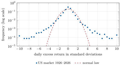
On 19 October 1987 the Dow Jones Industrial Average fell 22.6% in one session. The whole US stock market, value-weighted and in excess of bills, fell 17.4%: 22 times the standard deviation of its daily returns over the previous five years. Under a normal law such a day has a probability too small to be worth writing down; in a century of daily data it is one of 103 days beyond five standard deviations, where a normal law would expect 0.015. Real returns are not normal, and the ways in which they are not are regular enough to have a name. This chapter states the stylised facts of returns and measures them on a century of US data; it then builds the book’s synthetic equity market and checks which facts it reproduces and which it misses, because every later chapter that uses the simulator inherits both.
5.1 Heavy tails and aggregational Gaussianity
Definition 5.1 (Stylised fact)
A stylised fact is a statistical property of returns found, qualitatively, across many assets, markets and periods, stated without the precision that would make it specific to one of them.
Cont (2001) lists eleven. The first two are the absence of linear autocorrelation of returns beyond very short intraday horizons, and heavy tails: the tails of the return distribution decay like a power, with a tail index (One Quant Book 4, chapter 15) above two and below five for most data sets. The daily excess return of the US market from July 1926 to July 2026 (26 296 days, from the Kenneth French data library) has a kurtosis of 19.1; the Hill estimator on the 500 largest losses gives a tail index of 2.90, and on the 500 largest gains 2.58. Gopikrishnan and co-authors (1998) found an exponent of about three in forty million trade-by-trade price changes of US stocks, the “inverse cubic law”. Figure 5.1 shows the century’s daily returns against a normal law with the same standard deviation.
Definition 5.2 (Aggregational Gaussianity)
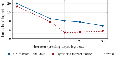
Aggregational Gaussianity is the tendency of returns summed over longer horizons to look more normal: their kurtosis falls towards three as the horizon grows, so that the shape of the distribution depends on the horizon.
The fall is slow (Figure 5.2). The kurtosis of the century’s log returns is 20.0 at one day, 11.5 at a week, 9.5 at a month and 7.3 at a quarter. Independent draws would bring a kurtosis of 20 down to in a month of 21 days; the returns are uncorrelated but not independent, and volatility clustering keeps the monthly tails heavy.
firm.synthmkt, seed 1.5.2 Volatility clustering and long memory in size
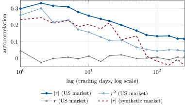
Returns are nearly uncorrelated: the century’s first-order autocorrelation is 0.046. Their sizes are not. Large moves follow large moves (volatility clustering, Book 4, chapter 18), and the dependence lasts: the autocorrelation of absolute returns is 0.30 at one day, 0.22 at twenty days and 0.13 at a hundred (Figure 5.3). Cont describes the decay as roughly a power of the lag with an exponent between 0.2 and 0.4, the long memory of Book 4, chapter 17.
Definition 5.3 (Taylor effect)
The Taylor effect is the finding that the autocorrelations of absolute returns exceed those of their powers for , in particular those of squared returns (Granger and Ding, 1996, after Taylor, 1986).
The century shows it at every lag: 0.30 against 0.26 at one day, 0.22 against 0.11 at twenty, 0.13 against 0.04 at a hundred. Squares give the largest moves too much weight, and the largest moves are the least persistent part of volatility. The practical consequence is modest but real: models and diagnostics of volatility persistence built on absolute returns see more of it than those built on squares.
firm.synthmkt, seed 1.5.3 The leverage effect and gain–loss asymmetry
Definition 5.4 (Gain–loss asymmetry)
Gain–loss asymmetry is the observation that stock prices and indices have large falls but not equally large rises: the distribution of returns is negatively skewed, and more so at horizons of weeks than of days.
The century’s daily skewness is ; over a week it is and over a month . The largest daily fall is the of 19 October 1987; the largest daily rise, on 15 March 1933, came in the most volatile market of the century. The leverage effect (Book 4, chapter 18), the negative correlation between returns and later volatility, is visible in the same data: the correlation between today’s return and tomorrow’s squared return is , against between today’s return and yesterday’s squared return. Falls raise volatility; volatility does not predict the sign of returns.
5.4 Intraday seasonality
Definition 5.5 (Intraday seasonality, intraday volume profile)
Intraday seasonality is the regular dependence of volatility, volume, spreads and trading activity on the time of day. The intraday volume profile is the average share of a day’s volume traded in each interval of the session.
Equity markets trade most, and move most, just after the open and just before the close: Wood, McInish and Ord (1985) found unusually high returns and standard deviations at the beginning and end of the day in minute-by-minute NYSE data, and Andersen and Bollerslev (1997) model this intraday periodicity jointly with the persistence of volatility from day to day. The pattern matters to anyone who samples in clock time: a return over the first five minutes of the day and one over five minutes at noon are draws from different distributions. The book’s intraday simulator builds the profile in (chapter 2): on its day the first quarter-hour trades 2.6 times the median quarter-hour’s volume and the last 1.7 times. The chapter has no licensed intraday data to measure it on real stocks; the profile of the simulator is an assumption, stated as one.
5.5 Cross-sectional structure
Stocks move together, and how much depends on the market’s direction.
Definition 5.6 (Exceedance correlation, correlation asymmetry)
An exceedance correlation is a correlation between returns measured only on the days when a conditioning variable (a market return, or the two returns themselves) lies beyond a threshold. Correlation asymmetry is the finding that exceedance correlations in falling markets exceed those in rising markets at the same threshold.
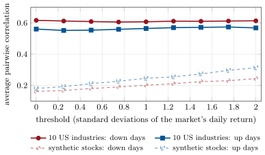
Longin and Solnik (2001) found, with extreme-value methods, that correlation between international equity markets increases in bear markets but not in bull markets; Ang and Chen (2002) found the same asymmetry between US stock portfolios and the market. The French data library’s ten industry portfolios show it over the century (Figure 5.4): on days when the market fell by more than one standard deviation their average pairwise correlation is 0.61; on days it rose as much, 0.56; the gap is there at every threshold from zero to two standard deviations. Diversification across industries is worth least on the days it is needed.
The second cross-sectional fact is a dominant factor. The correlation matrix of 200 simulated stocks over a year has a largest eigenvalue of 44.5, 22% of the total, against a Marchenko–Pastur upper edge of 3.58 for pure noise of the same shape (Book 4, chapter 22); four eigenvalues lie above the edge: the market and the strongest industries.
firm.synthmkt, seed 1.5.6 A scorecard for the book’s simulator
firm.synthmkt, the build of this chapter, generates the cross-section the rest of the book trades: a market factor with GJR-GARCH volatility and Student- shocks, industry and style factors, stocks with heterogeneous specific volatility, earnings jumps, and four planted sources of expected return. The table scores it against the century of US data on the facts of this chapter.
| real | synthetic (firm.synthmkt) | |||
| fact (daily returns) | US market | market | EW index | median stock |
| kurtosis | 19.1 | 20.5 | 18.0 | 8.7 |
| left tail index (Hill, largest 2%) | 2.90 | 2.83 | 2.88 | 3.35 |
| autocorrelation of , lag 1 | 0.30 | 0.23 | 0.25 | 0.10 |
| autocorrelation of , lag 20 | 0.22 | 0.21 | 0.22 | 0.08 |
| autocorrelation of , lag 100 | 0.13 | |||
| autocorrelation of , lag 1 | 0.05 | 0.01 | ||
| correlation of with | ||||
| kurtosis of monthly log returns | 9.5 | 3.8 | 3.9 | 3.5 |
Remark 5.7 (What the simulator can and cannot be used for)
The simulator reproduces the daily tails, the clustering over a month and the leverage effect, which is what the backtests, predictor measurements and risk models of this book need. It misses three facts: volatility memory beyond about fifty days (GARCH decays exponentially), the heavy tails of monthly returns (it has no crashes longer than a day), and correlation asymmetry. Research whose answer depends on them (tail hedging, drawdown risk over months, the value of diversification in a sell-off) must not be validated on it.
5.7 Tutorial: scoring a simulator
Goal. Compute the stylised facts of a return series, apply them to the century of US data and to the synthetic market, and fill in the scorecard. End state: the table above and Figures 5.2, 5.3 and 5.4.
The statistics. One function computes every row of the scorecard for one series; the Hill estimator is Book 4’s.
def facts(r) -> dict:
    """The scorecard statistics of one daily return series."""
    r = np.asarray(r, float)
    lr = np.log1p(r)
    m = len(lr) // 21
    k = max(20, int(0.02 * len(r)))
    return {"kurtosis": kurtosis(r), "hill_left": hill(-r, k)[0], "acf_abs_1": acf(np.abs(r), 1),
            "acf_abs_20": acf(np.abs(r), 20), "acf_abs_100": acf(np.abs(r), 100), "acf_r_1": acf(r, 1),
            "leverage_1": float(np.corrcoef(r[:-1], r[1:] ** 2)[0, 1]),
            "kurtosis_21": kurtosis(lr[: m * 21].reshape(m, 21).sum(axis=1))}
Listing 5.1. The scorecard of one return series. code/research/05-stylised-facts-of-returns/python/rs_stylised.py The market factor. GJR-GARCH(1,1): negative shocks raise tomorrow’s variance more than positive ones; the Student- shocks give the tails that clustering alone does not.
    def fundamentals_store(self) -> Store:
        s = Store()
        for f in self.fundamentals:
            s.put(f["pid"], f["field"], f["fiscal_end"], f["filed"], f["value"])
            if f["restated"] >= 0:
                s.put(f["pid"], f["field"], f["fiscal_end"], f["restated"], f["restated_value"])
        return s


def _student(rng, df, size):
    """Student-t draws scaled to unit variance."""
    return rng.standard_t(df, size) * math.sqrt((df - 2.0) / df)
Listing 5.2. The synthetic market factor. code/firm/synthmkt/firm_synthmkt.py - Run
synth_series()for the synthetic rows,french_summary()for the real one, andfig_stylised.py. The real statistics come fromrs_fetch_french.py, which keeps only derived statistics of the library’s data.
What to change next. Raise garch_beta to 0.96 and garch_alpha to 0.01 (same persistence, slower decay) and see the autocorrelation at lag 100 move; make betas larger on down days and look for correlation asymmetry, and for what it does to the mean return.
5.8 Build: the synthetic equity market
Purpose. The book’s cross-section with the truth attached. Chapters 6–15 measure predictors on it, Part IV backtests on it, Part V builds risk models and portfolios on it, and Books 8 and 9 run their equity strategy tutorials on it.
Interface. MarketConfig (size, length, seed; market, industry and style factor parameters; specific volatility; the four planted alpha strengths; delisting, merger, split, dividend and filing rules); simulate(cfg) returning a Panel: daily ret, price, volume, shares, listed; industry, beta, style_x, spec_vol; the factor paths and the market’s conditional variance; alpha (the planted expected return for the next day, by component); delistings, splits, dividends, earnings with their true surprises, point-in-time fundamentals with restatements; a secmaster.
Rules. Deterministic for a seed. The planted expected return for day is recorded at day , so that a signal known at the close of can be scored against it. A delisted name is replaced the next day. Fundamentals are filed after the quarter’s end and restatements come later still.
Acceptance tests. code/firm/synthmkt/tests/: determinism and bookkeeping (listed count, delisting returns, no return after a delisting); agreement with the security master; point-in-time fundamentals through firm.pit; over three seeds, market kurtosis above 5, positive volatility clustering at twenty days, a negative leverage correlation and positive reversal and momentum information coefficients; a dominant first eigenvalue.
Stretch. Downside betas with a compensating drift (correlation asymmetry); a slowly varying volatility component (long memory); multi-day crashes.
Sources and further reading
- R. Cont, “Empirical properties of asset returns: stylized facts and statistical issues”, Quantitative Finance 1(2), 2001.
- P. Gopikrishnan, M. Meyer, L. A. N. Amaral and H. E. Stanley, “Inverse cubic law for the distribution of stock price variations”, European Physical Journal B 3, 1998.
- C. W. J. Granger and Z. Ding, “Varieties of long memory models”, Journal of Econometrics 73, 1996; S. J. Taylor, Modelling Financial Time Series, Wiley, 1986.
- R. A. Wood, T. H. McInish and J. K. Ord, “An investigation of transactions data for NYSE stocks”, Journal of Finance 40(3), 1985; T. G. Andersen and T. Bollerslev, “Intraday periodicity and volatility persistence in financial markets”, Journal of Empirical Finance 4, 1997.
- F. Longin and B. Solnik, “Extreme correlation of international equity markets”, Journal of Finance 56(2), 2001; A. Ang and J. Chen, “Asymmetric correlations of equity portfolios”, Journal of Financial Economics 63(3), 2002.
- B. Mandelbrot, “The variation of certain speculative prices”, Journal of Business 36(4), 1963.
- Kenneth R. French, Data Library: Fama/French 3 factors and 10 industry portfolios, daily.
- Federal Reserve History, “Stock Market Crash of 1987”.
5.9 Exercises
Exercise 5.1 ★
A normal law with the century’s standard deviation of 1.08% a day: what is the probability of a day below , and how many such days would you expect in 26 296?
Solution
Solution of Exercise 5.1.
standard deviations; , so about such days in 26 296: never, in any number of universes’ lifetimes. It happened once.
Exercise 5.2 ★
If daily returns were independent with kurtosis 20, what would the kurtosis of their sum over 5, 21 and 63 days be? Compare with the century’s 11.5, 9.5 and 7.3.
Solution
Solution of Exercise 5.2.
For independent summands the excess kurtosis divides by the number of terms: , , . The century’s 11.5, 9.5 and 7.3 are far above: large moves cluster in time, so they do not average out.
Exercise 5.3 ★
A power-law tail with index 3: if one day in a thousand falls by more than 4%, how often does a day fall by more than 8%? And with an index of 4?
Solution
Solution of Exercise 5.3.
, so doubling the threshold divides the probability by : with , one day in 8 000 falls by more than 8%; with , one in 16 000.
Exercise 5.4 ★★
Show that for a Student- law with degrees of freedom, scaled to unit variance, the kurtosis is . What matches a kurtosis of 19?
Solution
Solution of Exercise 5.4.
For a Student- with degrees of freedom, and , so the kurtosis is , unchanged by scaling. A kurtosis of 19 needs , : barely more than four degrees of freedom.
Exercise 5.5 ★★
The ten industries have an average pairwise correlation of 0.61 on the market’s down days and 0.56 on its up days (one standard deviation). With equal weights and equal volatilities , what is the volatility of the equal-weighted portfolio relative to in each case?
Solution
Solution of Exercise 5.5.
The variance of an equal-weighted portfolio of 10 assets with volatility and pairwise correlation is : on down days and on up days. Diversification removes 19% of the volatility when the market falls and 22% when it rises.
Exercise 5.6 ★★
The GJR-GARCH market factor has , , . What is its persistence, and the half-life of a variance shock? Why does its autocorrelation of absolute returns fade after about fifty days?
Solution
Solution of Exercise 5.6.
Persistence (half the negative shocks carry ); a variance shock halves in days. The autocorrelation of absolute returns decays like the persistence raised to the lag, exponentially: small after a few half-lives, while the real series decays like a power of the lag.
Exercise 5.7 ★★★
Coding. Simulate the synthetic market with garch_alpha=0.01, garch_gamma=0.05, garch_beta=0.965 (the same persistence) and compare the autocorrelations of absolute market returns at lags 20 and 100 with the default’s.
Solution
Solution of Exercise 5.7.
With , , the persistence is exactly one (integrated GARCH): the autocorrelations of at lags 20 and 100 rise to 0.37 and 0.26, against 0.21 and for the default. But the variance no longer has a level to return to (the intercept is zero): over the ten years the conditional volatility wanders between 1.7% and 23.6% a year and the realised volatility is 7.7% instead of the intended 16%. Long memory needs another mechanism (a slow volatility component), not a unit root.
Exercise 5.8 ★★★
Find the flaw. “We validated our tail-hedging strategy on a simulated market calibrated to the daily kurtosis and volatility clustering of the S&P 500. It pays for itself over any ten-year window.”
Solution
Solution of Exercise 5.8.
A tail hedge pays in multi-day crashes and in sell-offs where correlations rise; a simulator calibrated to daily kurtosis and clustering misses both (the book’s reproduces daily tails but has monthly kurtosis 3.8 against 9.5 and no correlation asymmetry). Its tail events are single days, too short and too diversifiable, so the hedge’s value is mismeasured; and ten-year windows of one simulated path hold very few tail events. Validate on data with crashes, and on a simulator that reproduces the monthly tails.
5.10 Problem: Is the Simulator Realistic?
Problem 5.1
Weekend problem — a scorecard of the book’s synthetic market against a century of data
The century of daily US market excess returns (French data library, derived statistics) and firm.synthmkt with its default configuration (1 000 names, ten years, seed 1).
Part I — Tails.
- What are the daily kurtoses of the US market and of the synthetic market factor?
- What left tail indices does the Hill estimator give each on its largest 2% of losses?
- How many days of the century lie beyond five standard deviations, and how many would a normal law predict?
- How many standard deviations of the previous five years was 19 October 1987?
- What kurtosis does the synthetic median stock have, and why is it lower than the index’s?
Part II — Dependence.
- What are the autocorrelations of absolute returns at lags 1, 20 and 100, real and synthetic?
- Where does the synthetic market fail, and why?
- Does the synthetic market show the leverage effect? Compare the correlations of with .
- What are the kurtoses of monthly log returns, and what explains the gap?
- Does the century show the Taylor effect at lag 20?
Part III — The cross-section.
- What are the ten industries’ average correlations on down and up days at one standard deviation?
- What does the synthetic market give, and what does that mean?
- What is the largest eigenvalue of 200 synthetic stocks’ correlation over a year, its share, and the Marchenko–Pastur edge?
- How many eigenvalues lie above the edge, and what are they?
Part IV — Verdict.
- Which research of this book may use the simulator without reservation?
- Which research must not be validated on it?
- What single change would most improve it for a tail-risk study?
- State the named result: the scorecard’s three rows the simulator matches best and the three it misses.
- Why does a simulator used for research need a scorecard at all?
- In one sentence: what is a stylised fact good for?
Solution
Solution of Problem 5.1.
1. 19.1 and 20.5. 2. 2.90 and 2.83. 3. 103, against 0.015. 4. 22.0 (a fall of 17.4% with a prior standard deviation of 0.79%). 5. 8.7: a stock’s specific shocks have Student- tails with four degrees of freedom but only a part of its variance comes from the clustering market factor. 6. Real 0.30, 0.22, 0.13; synthetic market 0.23, 0.21, . 7. At lag 100: GARCH decays exponentially (half-life 69 days), the real series like a power. 8. Yes: against the real . 9. 9.5 against 3.8: the century’s crashes lasted weeks (1929–1933, 1987, 2008) and volatility regimes lasted years; the simulator has neither. 10. Yes: 0.22 for against 0.11 for . 11. 0.61 and 0.56. 12. 0.20 on down days and 0.25 on up days: the simulator orders them the wrong way, so it understates the cost of a crash to a diversified book. 13. 44.5, 22% of the total, against an edge of 3.58. 14. Four: the market and the strongest industry factors. 15. Predictor measurement, backtest mechanics, risk models at daily and weekly horizons, portfolio construction, costs. 16. Tail hedging, drawdowns over months, diversification in sell-offs, anything that depends on memory beyond fifty days. 17. Multi-day crashes with rising correlations (downside betas with a compensating drift, or a regime-switching volatility level). 18. Named result: the simulator matches the real daily kurtosis (20.5 against 19.1), the left tail index (2.83 against 2.90) and the clustering at twenty days (0.21 against 0.22); it misses the memory at a hundred days ( against 0.13), the monthly kurtosis (3.8 against 9.5) and the correlation asymmetry (0.20 down against 0.25 up, where the data give 0.61 against 0.56). 19. Because a result is only as realistic as the facts its data reproduce; the scorecard says which results transfer to markets. 20. It is a test that any model of returns, or any simulator, must pass before its conclusions are trusted.
5.11 Interview questions
Interview question 5.1 ★ researcher, trader
Name four stylised facts of equity returns.
Solution
Solution of Interview question 5.1.
Heavy tails (tail index about 3); no linear autocorrelation of returns but long-lasting autocorrelation of absolute returns (volatility clustering, long memory); the leverage effect; aggregational Gaussianity that is slow; gain–loss asymmetry; correlations that rise in sell-offs; intraday seasonality.
What the interviewer is looking for: several facts, with a number or a mechanism for each.
Interview question 5.2 ★★ researcher, risk
Daily returns are nearly uncorrelated. Does that make them independent? What would you check?
Solution
Solution of Interview question 5.2.
No: uncorrelated is not independent. Check the autocorrelations of and (volatility clustering), a test for ARCH effects, and whether kurtosis falls with aggregation as fast as independence predicts.
What the interviewer is looking for: the distinction, and a concrete test of nonlinear dependence.
Interview question 5.3 ★★ risk, researcher
Why does diversification across sectors disappoint in a crash?
Solution
Solution of Interview question 5.3.
Correlations are higher on down days than on up days (0.61 against 0.56 among US industries at one standard deviation), and volatility rises with them, so a diversified portfolio’s volatility is higher exactly when losses happen; the common market factor dominates in a sell-off.
What the interviewer is looking for: correlation asymmetry, not only rising volatility.
Interview question 5.4 ★★ researcher, mle
You want a simulator to test a trading strategy. How do you decide whether it is realistic enough?
Solution
Solution of Interview question 5.4.
Score it on the stylised facts that matter to the strategy: tails, clustering and its memory, leverage, correlation structure and its asymmetry, intraday seasonality if it trades intraday, against real data; then check that the strategy’s result does not depend on a fact the simulator misses (vary that feature and see if the answer moves).
What the interviewer is looking for: a scorecard tied to the strategy’s exposures.
Interview question 5.5 ★★★ researcher
If daily returns have kurtosis 20 and are independent, what is the kurtosis of monthly returns? The data say about 9. What does that tell you?
Solution
Solution of Interview question 5.5.
if independent. The observed 9 means that the daily returns are dependent in their sizes: large moves come in clusters that last weeks, so monthly returns inherit heavy tails; volatility clustering, not only heavy daily tails.
What the interviewer is looking for: the rule for excess kurtosis and the inference about dependence.
Interview question 5.6 ★★ trader, researcher
What is the leverage effect, and how would you measure it?
Solution
Solution of Interview question 5.6.
The negative correlation between returns and later volatility: falls raise volatility more than rises. Measure the correlation of with (or with realised volatility) for , against ; or fit an asymmetric GARCH and test .
What the interviewer is looking for: the direction of time in the measurement.