Research Craft: Predictors, Backtests, Measurement, Portfolios · Research

8Order-Book Features

Three lots rest at the best bid and forty at the best ask, the spread is one tick. Which way does the next mid-price change go? The book’s intraday simulator answers from three hours of its own data: when the bid queue is that much smaller, the next move is down three times in four. The order book is the most immediate information a market publishes, and every trading firm that acts at horizons of seconds reads it. This chapter defines the standard order-book features (imbalance at the touch and beyond, order-flow imbalance, the weighted mid and a microprice, queue depletion and cancellation rates), measures them on firm.tape, compares the imbalance with the prediction of a queueing model, and builds a streaming feature engine in three languages. Its data are three hours of simulated messages: 239 528 of them.

8.1 Imbalance at the touch

Definition 8.1 (Queue imbalance)

The queue imbalance at the touch is $I = (q^b - q^a)/(q^b + q^a)$ , where $q^b$ and $q^a$ are the quantities resting at the best bid and the best ask; it lies in $[-1, 1]$ and is positive when the bid queue is the larger.

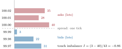
The book around the touch: three lots at the best bid (99.99), forty at the best ask (100.00). The queue imbalance at the touch is -0.86; over three levels on each side it is (56 - 103)/159 = -0.30, because the deeper bids are larger. A schematic, not data. — **Figure 8.1.** The book around the touch: three lots at the best bid (99.99), forty at the best ask (100.00). The queue imbalance at the touch is $-0.86$ ; over three levels on each side it is $(56 - 103)/159 = -0.30$ , because the deeper bids are larger. A schematic, not data.

When the spread is one tick, the mid moves only when one of the two best queues empties (or a new level appears inside a wider spread). A small bid queue is closer to emptying than a large ask queue, so imbalance predicts the direction of the next move. The first model of this is a race.

Proposition 8.2 (Imbalance as a race of two queues)

Model the two best queues, in lots, as independent birth–death processes with arrival rate $\lambda$ and departure rate $\mu$ (Book 4, chapter 8), starting from $q^b$ and $q^a$ . The probability that the next mid move is up is the probability that the ask queue empties first, $\int_0^\infty(1 - F_{q^b}(t))\,dF_{q^a}(t)$ , where $F_q$ is the law of the time for a queue starting at $q$ to empty. It increases with $q^b$ , decreases with $q^a$ , and equals $\tfrac12$ when $q^b = q^a$ .

Proof. The next move is up when the ask side empties before the bid side; with independent queues this is the stated race. A larger starting queue takes stochastically longer to empty, which gives the monotonicity; symmetry gives $\tfrac12$ . ∎

On the simulator’s three hours, 2.03 lots a second arrive at each best queue and 2.13 leave it (additions at the best price; cancellations and executions there). Figure 8.2 sets the race’s prediction against the data, bucket by bucket of the imbalance. The direction is right: the probability of an up move rises from 0.245 in the most ask-heavy tenth of observations to 0.736 in the most bid-heavy. The model is far too confident: it predicts 0.017 and 0.979. The reason is the mechanism the simulator plants, and that real markets share: the queues are not independent random walks, because the efficient price moves and the liquidity providers on its wrong side cancel. Imbalance is a noisy view of that, and a queueing model that ignores it overstates what the view is worth. Gould and Bonart (2016) fit the same relation by logistic regression on ten Nasdaq stocks and find a strongly significant improvement over a null model, large for large-tick stocks.

Probability that the next mid-price move is up, by tenth of queue imbalance at a one-tick spread: 0.245 to 0.736 in three hours of firm.tape, against 0.017 to 0.979 for the race of two independent birth–death queues with the rates measured on the same data. Data: firm.tape, seed 8; firm.queues. 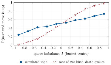— **Figure 8.2.** Probability that the next mid-price move is up, by tenth of queue imbalance at a one-tick spread: 0.245 to 0.736 in three hours of `firm.tape`, against 0.017 to 0.979 for the race of two independent birth–death queues with the rates measured on the same data. Data: `firm.tape`, seed 8; `firm.queues`.

8.2 Depth beyond the touch

Definition 8.3 (Depth imbalance, depth profile)

The depth imbalance over $L$ levels is $(\sum_{i \le L}q^b_i - \sum_{i \le L}q^a_i)/(\sum_{i\le L}q^b_i + \sum_{i \le L}q^a_i)$ , with $q^b_i, q^a_i$ the quantities at the $i$ -th best bid and ask prices. The depth profile of a side is the vector of its quantities by distance from the touch.

Depth beyond the touch is where the next best quote will come from once a queue empties, and where large orders show their hand, or hide it. Its information is slower than the touch’s and more easily faked (orders far from the touch are cheap to place and cancel, which Book 9, chapter 29, returns to). A depth profile is a feature vector rather than a number: its slope, its concentration, the distance to the first level holding more than a given quantity. The engine of this chapter computes the imbalance over the first five levels; the depth profile itself is the input of the machine-learned models of Book 12.

8.3 Order-flow imbalance

Definition 8.4 (Order-flow imbalance)

Let $b_n, q^b_n, a_n, q^a_n$ be the best bid, its size, the best ask and its size after the $n$ -th book event. The order-flow imbalance contribution of event $n$ is

e_n = \mathbf 1_{b_n \ge b_{n-1}}q^b_n - \mathbf 1_{b_n \le b_{n-1}}q^b_{n-1} - \mathbf 1_{a_n \le a_{n-1}}q^a_n + \mathbf 1_{a_n \ge a_{n-1}}q^a_{n-1},

and the order-flow imbalance (OFI) over an interval is the sum of the $e_n$ in it (Cont, Kukanov and Stoikov, 2014).

The four terms count demand added at the bid, demand removed from it, supply added at the ask and supply removed from it; when a price level changes, the whole old queue counts as removed and the whole new one as added. Cont, Kukanov and Stoikov found on 50 US stocks that over short intervals price changes are mainly driven by OFI, through a linear relation whose slope is inversely proportional to market depth.

Method 8.5 (Measuring the impact of order flow)

On a grid of intervals of length $\Delta$ , regress the change in mid price (in ticks) on the interval’s OFI divided by the average size of the best queues; the slope is the price impact per unit of depth-normalised flow, and the $R^2$ says how much of the price change the flow explains at that horizon.

On the simulated tape the regression explains 10% of mid changes at one second, 53% at ten seconds and 79% at sixty; the slope at ten seconds is 0.47 ticks per average best-queue size of net flow (Figure 8.3). At one second most intervals have no mid change at all, and those that do are single ticks triggered by the last event, which OFI sees only in part.

Mid-price change over ten-second intervals against the interval’s order-flow imbalance, in twenty bins of equal count, with the regression line (slope 0.47 ticks per unit, R2 = 0.53 on the 1 078 intervals). Data: firm.tape through firm.lobfeat, seed 8. — **Figure 8.3.** Mid-price change over ten-second intervals against the interval’s order-flow imbalance, in twenty bins of equal count, with the regression line (slope 0.47 ticks per unit, $R^2 = 0.53$ on the 1 078 intervals). 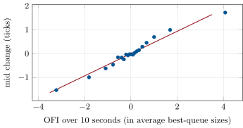Data: `firm.tape` through `firm.lobfeat`, seed 8.

8.4 The microprice

Definition 8.6 (Weighted mid price, microprice)

The weighted mid price is $(a\,q^b + b\,q^a)/(q^b + q^a)$ : the mid moved towards the side with the smaller queue. The book’s microprice is the mid plus the expected size and sign of the next mid change given the current imbalance bucket (at a one-tick spread), estimated on past data.

The weighted mid uses the imbalance through a fixed formula; the microprice learns the adjustment from data. Stoikov (2018) builds the full estimator from the whole sequence of later mid changes and finds it a better predictor of short-term prices than either the mid or the weighted mid; the book’s version keeps only the first term of that sequence. Fitted on the first half of the simulated session and scored on the second, it has a mean squared error 10% below the mid’s for the mid one second later; the weighted mid is 27% worse at one second but the best at five and thirty seconds (12% and 3% below the mid). A first-order correction is right about the next move and blind beyond it; the weighted mid is crude but keeps pointing the right way.

Mean squared error of the weighted mid and of the one-step microprice as forecasts of the mid 1, 5 and 30 seconds later, relative to the mid’s own error, on the second half of the simulated session (the microprice’s table is fitted on the first). Data: firm.tape through firm.lobfeat, seed 8. — **Figure 8.4.** Mean squared error of the weighted mid and of the one-step microprice as forecasts of the mid 1, 5 and 30 seconds later, relative to the mid’s own error, on the second half of the simulated session (the microprice’s table is fitted on the first). 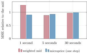Data: `firm.tape` through `firm.lobfeat`, seed 8.

8.5 Queue depletion and cancellations

Definition 8.7 (Queue depletion rate, cancellation rate)

The queue depletion rate of a best queue is the quantity leaving it per second (cancellations and executions) over a trailing window; its cancellation rate counts cancellations only.

Rates carry what sizes do not: a queue of forty lots losing ten a second is weaker than one of twenty losing none. In the simulator, liquidity providers cancel faster on the side the efficient price has moved away from, as real ones do when their quotes become stale. The difference between the cancellations at the best ask and at the best bid over the last second is therefore a direct view of the hidden price: its correlation with the direction of the next mid move is 0.30, against 0.25 for the queue imbalance. The general lesson is the chapter’s: the most informative features are those closest to the mechanism that moves the price.

8.6 Predictor cards

Predictor card 8.1 — Queue imbalance

Definition. $I = (q^b - q^a)/(q^b + q^a)$ at the touch, after each message.

Inputs and timestamps. The book after the last message received; the receive time is the knowledge time.

Rationale. The smaller queue empties first (Proposition 8.2); liquidity providers on the wrong side of the efficient price withdraw.

Horizon and half-life. The next mid move, seconds. P(up) from 0.245 to 0.736 across tenths of $I$ on the simulated tape.

Normalisation. None needed: bounded; bucketed or fed to a logistic model.

Failure modes. Spoofed size (Book 9, chapter 29); hidden and iceberg orders; wide spreads, where moves need not empty a queue.

Sources. Gould and Bonart (2016); rs_orderbook.up_probability.

Predictor card 8.2 — Order-flow imbalance

Definition. The sum of the $e_n$ over the last $\Delta$ seconds, divided by the average best-queue size.

Inputs and timestamps. Every book event, in sequence, with receive times.

Rationale. Net demand at the touch moves the price linearly, with a slope inversely proportional to depth.

Horizon and half-life. Contemporaneous in its definition; as a predictor, the next seconds. $R^2$ 10%, 53% and 79% at 1, 10 and 60 seconds (contemporaneous) on the simulated tape.

Normalisation. By depth; by volatility across instruments.

Failure modes. Needs every event in order (a gap in the feed corrupts the sum); spoofed additions count as demand.

Sources. Cont, Kukanov and Stoikov (2014); rs_orderbook.ofi_regression.

Predictor card 8.3 — Stale-quote cancellation imbalance

Definition. Lots cancelled at the best ask minus lots cancelled at the best bid over the last second.

Inputs and timestamps. Cancel messages with their prices and receive times.

Rationale. Liquidity providers pull quotes the efficient price has left behind.

Horizon and half-life. The next mid move; correlation 0.30 with its direction on the simulated tape.

Normalisation. By the queues’ sizes, or ranked across instruments.

Failure modes. Cancel-and-replace at the same price by an algorithm that refreshes its quotes; venue differences in how amendments are reported.

Sources. The simulator’s mechanism (chapter 2); rs_orderbook.cancel_feature.

8.7 Tutorial: reading the book

Goal. Run three hours of simulated messages through the feature engine, measure imbalance, OFI and the microprice, and compare the imbalance with the queueing model. End state: Figures 8.2, 8.3 and 8.4.

The engine. Apply the message to the order and level maps, read the new top, compute the OFI contribution from the previous top, then the imbalances, the weighted mid and the microprice.

    def on(self, kind: str, oid: int, side: int, price: int, qty: int):
        lv = self.book[side]
        if kind == "A":
            self.orders[oid] = [side, price, qty]
            lv[price] = lv.get(price, 0) + qty
        else:
            o = self.orders[oid]
            o[2] -= qty
            lv[price] -= qty
            if o[2] == 0:
                del self.orders[oid]
            if lv[price] == 0:
                del lv[price]
        top = self._top()
        if top is None:
            return None
        bb, qb, ba, qa = top
        e = 0
        if self.prev is not None:
            pb, pqb, pa, pqa = self.prev
            e = ((qb if bb >= pb else 0) - (pqb if bb <= pb else 0)
                 - (qa if ba <= pa else 0) + (pqa if ba >= pa else 0))
        self.prev = top
        self.ofi_cum += e
        imb = (qb - qa) / (qb + qa)
        db, da = self._depth(1), self._depth(-1)
        dimb = (db - da) / (db + da)
        mid = 0.5 * (bb + ba)
        wmid = (ba * qb + bb * qa) / (qb + qa)
        micro = mid + (self.g[bucket(imb, len(self.g))] if self.g and ba - bb == 1 else 0.0)
        return Features(bb, ba, qb, qa, imb, dimb, e, self.ofi_cum, wmid, micro)

Listing 8.1. One message through the Python reference engine. code/firm/lobfeat/firm_lobfeat.py

The race. The probability that the ask queue empties first, from the depletion laws of Book 4’s firm.queues, conditioned on one of them emptying within ten minutes.

def model_up_probability(qb: float, qa: float, birth: float, death: float, horizon: float = 600.0) -> float:
    """P(the ask queue empties before the bid queue) for independent birth-death queues in lots."""
    t = np.linspace(0.0, horizon, 1201)
    cdf_b = depletion_cdf(birth, death, max(1, round(qb)), t)
    cdf_a = depletion_cdf(birth, death, max(1, round(qa)), t)
    p = race(cdf_a, cdf_b, t)
    q = race(cdf_b, cdf_a, t)
    return p / (p + q)                                   # condition on a depletion within the horizon

Listing 8.2. The birth–death race. code/research/08-order-book-features/python/rs_orderbook.py

Run up_probability(), best_level_rates(), ofi_regression at 1, 10 and 60 seconds, forecast_errors(), cancel_feature() and fig_orderbook.py.

What to change next. Fit a logistic regression of the next move’s direction on $I$ and on the cancellation imbalance together; estimate the microprice table on spreads of two ticks as well.

8.8 Build: the streaming feature engine

Purpose. The order-book features of the miniature firm, computed message by message in the same way in research (Python) and in production (C++20, with a Rust twin); Book 11’s market maker and Book 12’s order-book model consume them.

Interface. Engine(levels, g).on(kind, oid, side, price, qty) returning Features (best quotes and sizes, imbalance, depth_imbalance, ofi, ofi_cum, wmid, micro); run(msgs); LobFeatures in cpp/firm_lobfeat.hpp and rust/src/lib.rs.

Rules. Integer prices and sizes; no features until both sides have a quote; the OFI of the first two-sided event is zero; identical arithmetic in the three languages.

Acceptance tests. code/firm/lobfeat/tests/: a hand-checked sequence of adds, executions and a level change; the committed fixture reproduced by the Python reference; bounded imbalances and OFI tracking the mid; the C++ and Rust tests replay the 2 769-message fixture and match every feature of the 2 766 two-sided rows.

Stretch. Depth profiles as fixed-size vectors; trailing-window depletion and cancellation rates in the engine; a lock-free single-writer queue feeding it (Book 13).

The C++ core, the one subtle part of the engine, is the order-flow update from the previous top of book:

        if (bids_.empty() || asks_.empty()) return std::nullopt;
        const std::int64_t bb = bids_.begin()->first, qb = bids_.begin()->second;
        const std::int64_t ba = asks_.begin()->first, qa = asks_.begin()->second;
        std::int64_t e = 0;
        if (has_prev_) {
            e = (bb >= pb_ ? qb : 0) - (bb <= pb_ ? pqb_ : 0) - (ba <= pa_ ? qa : 0) + (ba >= pa_ ? pqa_ : 0);
        }
        has_prev_ = true;
        pb_ = bb, pqb_ = qb, pa_ = ba, pqa_ = qa;
        ofi_cum_ += e;
        const double imb = static_cast<double>(qb - qa) / static_cast<double>(qb + qa);
        const std::int64_t db = depth(bids_), da = depth(asks_);
        const double dimb = static_cast<double>(db - da) / static_cast<double>(db + da);
        const double mid = 0.5 * static_cast<double>(bb + ba);
        const double wmid = static_cast<double>(ba * qb + bb * qa) / static_cast<double>(qb + qa);
        double micro = mid;
        if (!g_.empty() && ba - bb == 1) micro = mid + g_[bucket(imb, static_cast<int>(g_.size()))];
        return Features{bb, ba, qb, qa, imb, dimb, e, ofi_cum_, wmid, micro};

Listing 8.3. The C++20 engine after each message. code/firm/lobfeat/cpp/firm_lobfeat.hpp

Sources and further reading

R. Cont, A. Kukanov and S. Stoikov, “The price impact of order book events”, Journal of Financial Econometrics 12(1), 2014.
S. Stoikov, “The micro-price: a high-frequency estimator of future prices”, Quantitative Finance 18(12), 2018.
M. D. Gould and J. Bonart, “Queue imbalance as a one-tick-ahead price predictor in a limit order book”, Market Microstructure and Liquidity 2(2), 2016.
R. Cont, S. Stoikov and R. Talreja, “A stochastic model for order book dynamics”, Operations Research 58(3), 2010.
W. Huang, C.-A. Lehalle and M. Rosenbaum, “Simulating and analyzing order book data: the queue-reactive model”, Journal of the American Statistical Association 110(509), 2015.

8.9 Exercises

Exercise 8.1 ★

Best bid 99.98 for 700 shares, best ask 99.99 for 300. What are the queue imbalance, the mid and the weighted mid?

Solution

Solution of Exercise 8.1.

$I = (700 - 300)/1\,000 = 0.4$ ; the mid is 99.985; the weighted mid is $(99.99 \times 700 + 99.98 \times 300)/1\,000 = 99.987$ , moved towards the ask because the ask queue is the smaller.

Exercise 8.2 ★

The bid moves from 99.98 (500 shares) to 99.99 (200 shares) and the ask stays at 100.00 (400 shares, unchanged). What is the event’s OFI contribution?

Solution

Solution of Exercise 8.2.

The bid rose, so $+q^b_n = +200$ and the old bid queue is not subtracted; the ask did not change, so $-400 + 400 = 0$ : $e_n = +200$ .

Exercise 8.3 ★

The OFI slope is 0.47 ticks per average best-queue size, and that size is 2 750 shares. What mid move does a net buying flow of 11 000 shares over ten seconds predict?

Solution

Solution of Exercise 8.3.

$11\,000/2\,750 = 4$ average queue sizes; $4 \times 0.47 = 1.88$ ticks.

Exercise 8.4 ★★

For the race with $\lambda = \mu$ and queues of one lot at the bid and $n$ lots at the ask, argue that the probability of an up move tends to zero as $n$ grows. What does that say about the model’s extreme buckets?

Solution

Solution of Exercise 8.4.

With $\lambda = \mu$ a queue of $n$ lots takes a time to empty that grows without bound in probability as $n$ grows, while the one-lot queue empties in a time that does not depend on $n$ ; so the ask almost surely survives the bid, and P(up) tends to zero. The model’s extreme buckets are therefore near 0 and 1, whereas the data stay between 0.25 and 0.74: something other than the queues’ own random walks moves the price.

Exercise 8.5 ★★

Why does OFI’s $R^2$ rise with the length of the interval, from 10% at one second to 79% at sixty?

Solution

Solution of Exercise 8.5.

At one second most intervals have no mid change, and a change is a single tick set off by one event, of which OFI sees only part; over longer intervals the changes are sums of many events, their discreteness averages out, and the linear relation with the summed flow shows.

Exercise 8.6 ★★

Show that the weighted mid equals the mid plus $\tfrac s2 I$ , with $s$ the spread and $I$ the queue imbalance.

Solution

Solution of Exercise 8.6.

$(a q^b + b q^a)/(q^b + q^a) = \frac{a + b}{2} + \frac{a - b}{2}\cdot\frac{q^b - q^a}{q^b + q^a} = m + \frac s2 I$ .

Exercise 8.7 ★★★

Coding. Using the tape of the chapter, compute the correlation of the depth imbalance over five levels with the direction of the next mid move, and compare it with the touch imbalance’s.

Solution

Solution of Exercise 8.7.

0.277 for the five-level depth imbalance against 0.253 for the touch imbalance: the deeper levels add information here because the simulator’s liquidity providers also cancel stale quotes behind the touch. On real data the deeper levels are also where orders are cheapest to fake.

Exercise 8.8 ★★★

Find the flaw. “Our order-book model predicts the next mid move with 74% accuracy. We computed the features from the consolidated book stamped with exchange timestamps and the target from the same feed.”

Solution

Solution of Exercise 8.8.

The features must be computed at the time the firm could have them, the receive time, not the exchange time; and a consolidated book built on exchange timestamps assumes all venues’ messages arrive at once, which they do not. The accuracy is also uninformative without the base rate: at extreme imbalances the naive direction is already right three times in four. Recompute with receive-time books and report the accuracy by bucket against the base rate.

8.10 Problem: Three Lots Against Forty

Problem 8.1

Weekend problem — how much does the order book know, and how much does a queueing model think it knows?

Three hours of firm.tape (seed 8), 239 528 messages, through firm.lobfeat.

Part I — Imbalance.

What are the probabilities of an up move in the lowest and highest tenths of the queue imbalance?
How many observations fall in each of those two tenths?
What are the average queue sizes (lots) in the extreme tenths?
At what imbalance is the probability one half?

Part II — The model.

What arrival and departure rates (lots per second) does each best queue have?
What does the race predict for the extreme tenths?
Why is the model too confident?
Which mechanism of the simulator would a correct model have to include?

Part III — Flow.

What are OFI’s $R^2$ at 1, 10 and 60 seconds, and its slope at ten seconds?
What is the average best-queue size used to normalise it?
How does the one-step microprice compare with the mid at one second?
Which forecast wins at five and thirty seconds, and by how much?
What is the cancellation imbalance’s correlation with the next move, and the queue imbalance’s?

Part IV — Engineering and judgement.

Why must the three implementations of the engine produce identical numbers?
How many fixture rows do the C++ and Rust tests check?
Which features need every message in sequence, and which survive a snapshot feed?
Which of the chapter’s features would a spoofer move most easily?
State the named result: the empirical and modelled probabilities of an up move in the extreme tenths of imbalance, and OFI’s $R^2$ at ten seconds.
What would you add to the race model first?
In one sentence: what does the order book tell you?

Solution

Solution of Problem 8.1.

1. 0.245 and 0.736. 2. 16 564 and 14 538. 3. 3.4 against 55.4 lots, and 49.2 against 3.1. 4. Near zero, slightly below (the bucket centred on $-0.1$ gives 0.500). 5. 2.03 lots a second arrive and 2.13 leave. 6. 0.017 and 0.979. 7. It treats the queues as independent random walks, while the efficient price drives which side is cancelled and traded against, and new liquidity keeps arriving at the smaller queue. 8. The efficient price: informed orders and stale-quote cancellations that depend on where it is. 9. 10%, 53% and 79%; 0.47 ticks per average best-queue size. 10. 2 747 shares (27.5 lots). 11. A mean squared error 10% below the mid’s. 12. The weighted mid: 12% and 3% below the mid. 13. 0.30 and 0.25. 14. Because a model researched on one set of numbers and traded on another is a different model; any discrepancy is a silent bug. 15. 2 766 two-sided rows of 2 769 messages. 16. OFI and the rates need every event in order; the imbalances, the weighted mid and the microprice can be computed from snapshots. 17. Depth beyond the touch, and the touch imbalance itself: orders placed without intent to trade. 18. Named result: across tenths of queue imbalance the probability of an up move runs from 0.245 to 0.736 on the simulated tape, where the race of two birth–death queues predicts 0.017 to 0.979; OFI explains 53% of ten-second mid changes. 19. The efficient price: arrivals and cancellations that depend on it (a queue-reactive model with a hidden state). 20. Where supply and demand stand right now, and, with its flow, where the price is about to go.

8.11 Interview questions

Interview question 8.1 ★ trader, researcher

The bid queue is ten times the ask queue at a one-tick spread. What do you expect the next price move to be, and why?

Solution

Solution of Interview question 8.1.

Most likely up: the small ask queue is much closer to emptying, and liquidity providers on the ask may be the ones withdrawing. But not with the certainty a naive queue race suggests; on the simulated tape the most bid-heavy tenth gives about 0.74, not 0.98.

What the interviewer is looking for: direction plus calibration: imbalance is informative but noisy.

Interview question 8.2 ★★ researcher

Define order-flow imbalance and explain why it relates linearly to price changes.

Solution

Solution of Interview question 8.2.

Net quantity added at the bid, minus removed from it, minus added at the ask, plus removed from it, counting whole queues when prices change. A net order flow of size $x$ consumes or builds queues of typical size $D$ ; the price moves by about one tick per queue consumed, so the change is proportional to $x/D$ : linear, with a slope inversely proportional to depth.

What the interviewer is looking for: the four terms and the depth argument.

Interview question 8.3 ★★ researcher, developer

What is a microprice? How would you estimate one?

Solution

Solution of Interview question 8.3.

An estimate of the fair price better than the mid, using the imbalance (and spread): the expected future mid given the book. Estimate by bucketing the imbalance (and spread) and averaging subsequent mid changes, one step or iterated to convergence, on past data; validate out of sample against the mid and the weighted mid.

What the interviewer is looking for: conditioning on the state, estimation out of sample, the comparison.

Interview question 8.4 ★★ developer

Your research features are in Python and production is in C++. How do you guarantee they compute the same thing?

Solution

Solution of Interview question 8.4.

One reference implementation and a shared fixture: replay the same recorded messages through each implementation and require identical outputs (to the last bit where possible, to a tight tolerance otherwise) in continuous integration, with the same operation order in the arithmetic.

What the interviewer is looking for: a replay test on a shared fixture, not code review.

Interview question 8.5 ★★ trader, researcher

How can an order-book feature be manipulated, and how would you make a model robust to it?

Solution

Solution of Interview question 8.5.

Size shown and withdrawn without intent to trade moves imbalance and depth features (spoofing, layering); flow features count those additions as demand. Robustness: weight quantities by how long they rest or by the probability they trade, discount levels beyond the touch, use executed flow as well as quoted size, and monitor for sequences of large adds and cancels.

What the interviewer is looking for: the mechanism and at least two defences.

Interview question 8.6 ★★★ researcher

Model the best bid and ask queues as independent birth–death processes. What does the model predict for the next move, and what does it leave out?

Solution

Solution of Interview question 8.6.

P(up) is the probability that the ask queue empties first, increasing in the bid size and decreasing in the ask size; with equal rates it is one half at equal sizes. It leaves out the efficient price (informed flow and stale-quote cancellations that make depletions dependent on it), queue-reactive rates, and new levels inside the spread; it is therefore overconfident at extreme imbalances.

What the interviewer is looking for: the race, its monotonicity, and what makes it overconfident.

Terms defined in this chapter

See all 2333 terms in the glossary