Research Craft: Predictors, Backtests, Measurement, Portfolios · Research

24Risk Models

A market-neutral book is forecast at 3.3 per cent annual volatility and realises 9.2. Its risk model knew the market, ten industries, beta, size and value, and the book was neutral to all of them; it did not know momentum, and the book’s proprietary score, without anyone having checked, was half momentum. Over eight years its standardised returns have a standard deviation of 2.86 instead of one. The same book under a model that includes momentum is forecast at 9.23 per cent and realises 9.20. A risk model is a research tool before it is a reporting one: it says which risks a book takes, and it can only say so for the risks it knows. This chapter builds firm.riskmodel, a fundamental equity model in the style that commercial vendors describe publicly, fits it and a statistical model to firm.synthmkt, and evaluates them the way they should be evaluated, with bias statistics.

24.1 Three families of factor models

A factor model (Book 4, chapter 22) writes each stock’s return as exposures times factor returns plus a specific return. Models differ in what they observe.

Definition 24.1 (Fundamental, statistical and hybrid factor models; factor exposure, factor return, specific return)

In a fundamental factor model the factor exposures are observed characteristics of each stock (industry membership, standardised style scores) and the factor returns are estimated each period by cross-sectional regression. In a statistical factor model both are estimated from the returns alone, by principal components or factor analysis. A hybrid factor model adds statistical factors to a fundamental model to capture what its characteristics miss. The specific return is what the factors leave: the regression residual. (A third family, macroeconomic models, observes factor returns such as inflation or the term spread and estimates exposures by time-series regression.)

Definition 24.2 (Style factor, industry factor)

An industry factor has as exposure a stock’s membership of an industry; a style factor has as exposure a standardised characteristic (size, value, momentum, an estimated beta), cap-weighted to mean zero and scaled to unit cross-sectional standard deviation.

Rosenberg showed in 1974 that the covariance of stock returns has components beyond the market and that their loadings follow observable characteristics: the origin of the fundamental model. Connor compared the three families on US returns; Chen, Roll and Ross priced macroeconomic factors. The chapter’s model is fundamental, the family commercial vendors document: for their US model, MSCI describes a Country factor that makes the industry factors dollar-neutral (each industry measured net of the market), specific risk estimated from daily time series and shrunk within size groups, and a volatility regime adjustment.

24.2 Estimating factor returns

Each day $t$ the model regresses the cross-section of returns on the exposures known at the previous close:

\min_{f}\ \sum_i w_i\,(r_{it} - x_{i,t-1}^\top f)^2 \quad\text{subject to}\quad \sum_k c_k f_{k} = 0 \text{ over the industries},

with weights $w_i$ the square root of capitalisation (larger stocks have smaller specific variance) and $c_k$ the capitalisation share of industry $k$ . The country factor’s exposure is one for every stock, so the industry dummies alone would be collinear with it; the constraint makes the country factor the cap-weighted market and each industry factor its return net of the market. firm.riskmodel.cs_regression solves the constrained problem through its Karush–Kuhn–Tucker system (Listing 24.1).

On firm.synthmkt’s ten years, 1 000 listed names a day, the model has fifteen factors: country, ten industries, and four styles, each known at the previous close: beta, estimated over the trailing year and re-estimated monthly; size, the simulation’s latent characteristic, fixed at listing; value, the log of book to price from the latest filed book value (firm.synthmkt.point_in_time_styles); momentum, the 12–1 month return, reset every month. The country factor’s annual volatility is 17.8%, the industries’ between 8.0% and 8.7%, momentum’s 7.2%. The average daily cross-sectional $R^2$ is 0.19: most of a stock’s daily variance is specific, which is why a book of a hundred names a side still has specific risk worth modelling.

Point in time matters here as everywhere. The simulation keeps each stock’s style exposures up to date in place; a first version of this chapter’s model read them at the end of the sample and used them for all ten years. It fitted without complaint, and its momentum factor had a volatility of 3.3% instead of 7.2%: exposures from the future describe a different, smoother factor.

24.3 Factor covariance

The factor covariance forecast is an exponentially weighted estimate of the factor returns, with a half-life of 90 days (Book 4, chapter 18, for the exponentially weighted volatility). For horizons longer than a day, Newey–West terms add the autocovariances. Two refinements address the estimate’s two known failures. Volatility is not stationary: a backward-looking estimate lags when volatility rises. And sampling error makes the estimated covariance too confident about some directions, which an optimiser then finds (Menchero, Wang and Orr: optimised portfolios’ risk is underpredicted; chapter 25).

Definition 24.3 (Bias statistic, volatility regime adjustment)

The bias statistic of a portfolio’s risk forecasts over $T$ periods is the standard deviation of its standardised returns $r_t/\hat\sigma_{t-1}$ ; it is one for correct forecasts, within $1 \pm \sqrt{2/T}$ with probability about 95% for normal returns. The cross-sectional bias of day $t$ is $B_t^2 = \frac1K\sum_k f_{kt}^2/\hat\sigma_{k,t-1}^2$ over the factors. A volatility regime adjustment multiplies the covariance forecast by an exponentially weighted average $\lambda_t^2$ of recent $B_t^2$ , raising all factor volatilities together when the day’s factor returns are large for their forecasts.

The chapter’s adjustment uses a half-life of 42 days (Listing 24.2). The simulated market’s volatility follows a GJR-GARCH process, so regimes come and go. On the cap-weighted market portfolio the overall bias statistic is 1.00 without the adjustment and 0.99 with it; the difference is in the regimes. One-year rolling bias statistics range from 0.50 to 1.55 without it and from 0.56 to 1.32 with it, and 66% of the one-year windows fall outside their band ( $\pm 0.089$ ) without it against 44% with it (Figure 24.2). A year is still a long time for a GARCH market; a desk that trades on daily risk wants the adjustment and a short half-life.

24.4 Specific risk

Definition 24.4 (Specific risk)

A stock’s specific risk is the forecast standard deviation of its specific return.

Each stock’s specific variance is forecast by an exponentially weighted average of its squared residuals (half-life 90 days). Such forecasts are noisy, and noise sorts: the stocks forecast most volatile are, on average, those whose recent residuals were luckily large. Standardising each stock’s next-day residual by its forecast and grouping by the forecast’s decile shows it: the bias statistic is 1.13 in the lowest decile and 0.93 in the highest. Shrinking each forecast volatility 10% of the way towards the mean of its size decile, as MSCI describes for its model, flattens the pattern to between 0.97 and 1.04 (Figure 24.1). The remaining level, slightly above one, is the simulation’s Student- $t$ shocks and earnings-day jumps.

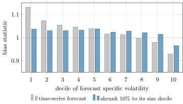
Bias statistics of next-day specific returns standardised by their forecasts, by decile of the forecast, years 3 to 10. Data: rs_riskmodel.specific_deciles. — **Figure 24.1.** Bias statistics of next-day specific returns standardised by their forecasts, by decile of the forecast, years 3 to 10. Data: `rs_riskmodel.specific_deciles`.

24.5 Evaluating a risk model

A portfolio’s forecast variance is $x^\top F x + \sum_i w_i^2 s_i^2$ , with $x = X^\top w$ its factor exposures, $F$ the factor covariance and $s_i^2$ the specific variances; each factor’s contribution $x_k (Fx)_k$ sums to the factor part (Listing 24.3). A model is judged by how its forecasts of many portfolios’ risk compare with what happened, not by the fit of its regression.

The chapter’s test portfolios are held from each close over the next day and rebuilt monthly, and are scored over years 3 to 10 (2 016 days; the bias band is $1 \pm 0.031$ ). Fifty random market-neutral books, a hundred names a side, have bias statistics between 0.96 and 1.04, averaging 1.00; 92% fall in the band (98% without the regime adjustment, which does nothing for books whose risk is mostly specific, and a little harm). The book of the opening is built from a score equal to 0.5 times the momentum score plus $\sqrt{0.75}$ times noise, long the top hundred and short the bottom hundred, then neutralised to every factor of the model without momentum. On day 1 500 the full model forecasts it at 6.88% a year, 76% of the variance from its momentum exposure of 1.03; over the eight years its exposure has a root mean square of 1.23.

the exposed book, years 3 to 10	forecast	realised	bias statistic
fundamental model, all factors	9.23%	9.20%	1.04
fundamental model without momentum	3.26%	9.20%	2.86
statistical model, 15 principal components	5.59%	9.20%	1.68

The model without momentum sees only the book’s specific risk; the momentum factor’s 7.2% volatility times the book’s exposure is the missing two thirds. The statistical model, fifteen principal components refitted monthly on the trailing year, finds part of it without being told (5.59%, a bias statistic of 1.68): momentum’s returns are a direction of common variation, which principal components look for, but its loadings are reset every month while a trailing year’s components assume loadings that stay put, so the direction the year’s data describe is an average of twelve different ones. A statistical model is still worth running beside the fundamental one as an alarm: here it forecasts 5.59% where the fundamental model says 3.26%, and when a book’s risk under the two models diverges, the fundamental model is missing something the book holds. That is the case for hybrid models too.

One-year rolling bias statistics. Left: the book exposed to momentum under the three models. Right: the cap-weighted market under the full model, with and without the volatility regime adjustment. Data: rs_riskmodel. — **Figure 24.2.** One-year rolling bias statistics. Left: the book exposed to momentum under the three models. Right: the cap-weighted market under the full model, with and without the volatility regime adjustment. 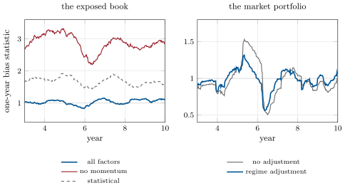Data: `rs_riskmodel`.

Bias statistics have their own uncertainty. Over sixty months the band is $1 \pm 0.18$ ; with fat tails fewer than 95% of correct forecasts fall inside it (MSCI reports 86% at a kurtosis of 5 over 120 periods). A single portfolio’s bias statistic is weak evidence; many portfolios, rolling windows and the portfolios the firm actually trades are what a model is judged on.

24.6 Tutorial: predicted three, realised nine

Goal. Fit a fundamental model with and without momentum and a statistical model to firm.synthmkt, forecast the risk of books out of sample, and evaluate by bias statistics. End state: the table, Figures 24.2 and 24.1.

The daily regression with the industry constraint.

def cs_regression(r, X, w, C=None):
    """Weighted least squares with linear equality constraints C f = 0, by the KKT system. Rows with NaN return or
    zero weight are ignored; residuals are NaN there."""
    r, X, w = np.asarray(r, float), np.asarray(X, float), np.asarray(w, float)
    ok = np.isfinite(r) & (w > 0) & np.all(np.isfinite(X), axis=1)
    Xo, ro, wo = X[ok], r[ok], w[ok]
    A = Xo.T @ (wo[:, None] * Xo)
    b = Xo.T @ (wo * ro)
    K = X.shape[1]
    if C is None or len(C) == 0:
        f = np.linalg.lstsq(A, b, rcond=None)[0]
    else:
        C = np.atleast_2d(np.asarray(C, float))
        kkt = np.block([[A, C.T], [C, np.zeros((len(C), len(C)))]])
        f = np.linalg.lstsq(kkt, np.r_[b, np.zeros(len(C))], rcond=None)[0][:K]
    e = np.full(len(r), np.nan)
    e[ok] = ro - Xo @ f
    return f, e

Listing 24.1. Constrained weighted cross-sectional regression. code/firm/riskmodel/firm_riskmodel.py

The volatility regime adjustment.

def vra(F, covs, half_life: float = 42.0):
    """lambda_t^2 = EWMA over s <= t of B_s^2, B_s^2 = mean_k f_ks^2 / var_k(forecast made at s - 1): scale the factor
    covariance forecast made at t by lambda_t^2 (volatility regime adjustment)."""
    F = np.asarray(F, float)
    T, _ = F.shape
    lam = 0.5 ** (1.0 / half_life)
    out, x = np.ones(T), 1.0
    for t in range(1, T):
        b2 = float(np.mean(F[t] ** 2 / np.diag(covs[t - 1])))
        x = lam * x + (1 - lam) * b2
        out[t] = x
    return out

Listing 24.2. The multiplier from the cross-sectional bias statistic. code/firm/riskmodel/firm_riskmodel.py

Portfolio risk and its decomposition.

def portfolio_risk(w, X, Fcov, spec):
    w, X, Fcov, spec = (np.asarray(a, float) for a in (w, X, Fcov, spec))
    x = X.T @ w
    contrib = x * (Fcov @ x)
    fac = float(contrib.sum())
    sp = float(np.nansum(w * w * spec))
    return {"total": fac + sp, "factor": fac, "specific": sp, "contrib": contrib, "exposure": x}

Listing 24.3. Factor and specific variance, and each factor’s contribution. code/firm/riskmodel/firm_riskmodel.py

Run rs_riskmodel.fundamental(), fundamental with momentum omitted, statistical(), summary(), random_bias(), market_bias(), specific_deciles() and fig_riskmodel.py.

What to change next. Drop the value factor instead of momentum and build a book exposed to it; add three principal components of the fundamental model’s residuals as statistical factors (a hybrid model) and see whether the missing factor comes back.

24.7 Build: an equity risk model

Purpose. The firm’s equity risk model: exposures, factor returns, covariance and specific risk every day, the risk of any book and its decomposition, and the evidence (bias statistics) that the forecasts are right.

Interface. cs_regression(r, X, w, C), factor_returns(R, exposures, W, C), ewma_cov(F, half_life, nw_lags), vra(F, covs, half_life), specific_var(E, half_life, groups, shrink), portfolio_risk(w, X, Fcov, spec), pca_model(R, k), bias_stat(r, sigma), bias_band(T).

Rules. Exposures known at the previous close; forecasts made at the close for the next period; every model change is judged on the bias statistics of random books, of the factor portfolios and of the books the firm holds; a statistical model runs beside the fundamental one.

Acceptance tests. code/firm/riskmodel/tests/: a constrained regression that recovers planted factor returns and satisfies its constraint; the covariance and the regime multiplier catching a planted volatility shift; specific variances recovering a planted level, shrinkage narrowing their dispersion; contributions summing to the factor variance; orthonormal principal components; bias statistics of known forecasts and the band.

Stretch. The eigenfactor adjustment of optimised portfolios’ risk; hybrid statistical factors; multi-day horizons with Newey–West terms.

Sources and further reading

B. Rosenberg, “Extra-market components of covariance in security returns”, Journal of Financial and Quantitative Analysis 9(2), 1974.
G. Connor, “The three types of factor models: a comparison of their explanatory power”, Financial Analysts Journal 51(3), 1995.
N.-F. Chen, R. Roll and S. A. Ross, “Economic forces and the stock market”, Journal of Business 59(3), 1986.
Y. Liu, J. Menchero, D. J. Orr and J. Wang, The Barra US Equity Model (USE4): Empirical Notes, MSCI, 2011.
J. Menchero, J. Wang and D. J. Orr, “Improving risk forecasts for optimized portfolios”, Financial Analysts Journal 68(3), 2012.

24.8 Exercises

Exercise 24.1 ★

A book’s forecast volatility is 3.26% from specific risk only. Its exposure to an omitted factor of 7.2% volatility has a root mean square of 1.23. What should its realised volatility be, and what bias statistic follows?

Solution

Solution of Exercise 24.1.

$\sqrt{3.26^2 + (1.23 \times 7.2)^2} = 9.4\%$ , against the realised 9.2%; the bias statistic is about $9.4/3.26 = 2.9$ (the measured one is 2.86).

Exercise 24.2 ★

Give the 95% band of the bias statistic for 60 monthly observations and for 2 016 daily ones.

Solution

Solution of Exercise 24.2.

$1 \pm \sqrt{2/60} = 1 \pm 0.18$ ; $1 \pm \sqrt{2/2\,016} = 1 \pm 0.031$ .

Exercise 24.3 ★

Why does a model with a country factor and a full set of industry dummies need a constraint, and what does the cap-weighted constraint make the factors mean?

Solution

Solution of Exercise 24.3.

The industry dummies sum to the country factor’s exposure (one for every stock), so the regression is singular: any constant can move between the country factor and the industries. Constraining the cap-weighted industry returns to zero makes the country factor the cap-weighted market and each industry factor the industry’s return net of the market (a dollar-neutral industry portfolio).

Exercise 24.4 ★★

Explain why time-series forecasts of specific volatility overpredict the high-volatility stocks and underpredict the low ones, even when each stock’s volatility is constant.

Solution

Solution of Exercise 24.4.

Each forecast is the true variance plus estimation noise. Sorting by the forecast sorts partly by the noise: the top decile holds the stocks whose recent residuals were luckily large (true variance below the forecast), the bottom those luckily small. The realised variance regresses to the true one, so the top decile is overpredicted (0.93) and the bottom underpredicted (1.13). Shrinking towards a group mean undoes part of the sort.

Exercise 24.5 ★★

The regime adjustment improved the market portfolio’s rolling bias statistics and slightly worsened the random books’. Why?

Solution

Solution of Exercise 24.5.

The adjustment scales the factor covariance by the recent cross-sectional bias of the factors. The market portfolio’s risk is almost all factor risk, whose regimes the adjustment tracks. The random books’ risk is mostly specific; they gain nothing, and inherit the multiplier’s noise on their small factor part.

Exercise 24.6 ★★

Show that the factor contributions $x_k(Fx)_k$ sum to the factor variance. Can a contribution be negative?

Solution

Solution of Exercise 24.6.

$\sum_k x_k (Fx)_k = x^\top F x$ . A contribution is negative when the exposure to a factor hedges the others: $x_k$ and $(Fx)_k$ of opposite signs.

Exercise 24.7 ★★★

Coding. Build the exposed book from a score loading 0.3 instead of 0.5 on momentum, and report the three models’ bias statistics.

Solution

Solution of Exercise 24.7.

Run rs_riskmodel.summary(0.3). The momentum exposure falls, so the model without momentum underpredicts less: bias statistics of 1.98 without momentum, 1.02 with all factors and 1.48 for the statistical model (realised volatility 6.53%, forecast 3.34% without momentum).

Exercise 24.8 ★★★

Find the flaw. “Our risk model explains only 19% of daily return variance, so it is useless for a book of two hundred names.”

Solution

Solution of Exercise 24.8.

The $R^2$ is about single stocks, whose daily variance is mostly specific. A book’s risk is the factor part, which does not diversify, plus a specific part that falls with the number of names; the model’s value is in forecasting both, measured by bias statistics (1.04 on the exposed book, 1.00 on average for random books), not by the regression’s fit.

24.9 Problem: Predicted Three, Realised Nine

Problem 24.1

Weekend problem — a model that did not know

The chapter’s models on firm.synthmkt.

Part I — The model.

List the fifteen factors and how each exposure is obtained.
Why square-root-of-capitalisation weights?
What are the factor volatilities of the country, the industries and momentum?
What is the average cross-sectional $R^2$ , and what does it mean for a book’s risk?

Part II — Covariance and specific risk.

How does the volatility regime adjustment work, and what does it do to the market portfolio’s rolling bias statistics?
Why does it not help the random books?
What pattern do raw specific forecasts show by decile, and what does shrinkage do?
Why does a residual level slightly above one remain?

Part III — The exposed book.

How is the exposed book built?
What are its forecasts, realised volatility and bias statistics under the three models?
What share of its forecast variance comes from momentum, at what exposure?
Why does the statistical model find most of the missing risk, but not all?

Part IV — The verdict.

State the named result: the bias statistic of the model missing the planted factor, and the realised-to-predicted volatility ratio of the exposed book.
How would the desk have found out before the drawdown?
What evidence would you require before adopting a new risk model?
How do fat tails change the reading of a bias statistic?
What is a hybrid factor model, and when is it worth building?
Why are the random books’ bias statistics a necessary but insufficient test?
Which book should a risk manager test first?
In one sentence: what does a risk model know?

Solution

Solution of Problem 24.1.

Country (one for every stock); ten industries (membership); beta (trailing-year regression on the cap-weighted market, monthly); size, value, momentum (size fixed at listing; value from the latest filed book; momentum from the 12–1 month return; all known at the previous close).
Specific variance falls with capitalisation; the weights approximate generalised least squares and give the country factor the cap-weighted market’s meaning.
17.8%; between 8.0% and 8.7%; 7.2%.
0.19: a stock’s daily variance is mostly specific, so specific risk matters even in a book of two hundred names.
It multiplies the factor covariance by an exponentially weighted average of the cross-sectional bias; the market’s rolling one-year bias statistics range over 0.56–1.32 instead of 0.50–1.55, and 44% of windows fall outside the band instead of 66%.
Their risk is mostly specific; the random books’ share inside the band is 92% with it and 98% without.
1.13 in the lowest decile to 0.93 in the highest; shrinking 10% towards the size decile’s mean gives 0.97 to 1.04.
The Student- $t$ shocks and earnings-day jumps of the simulation, which an exponentially weighted variance reflects late.
A score of 0.5 times the momentum score plus $\sqrt{0.75}$ times noise; the top and bottom hundred names; neutralised to the model without momentum; gross 2; rebuilt monthly.
All factors: 9.23% forecast, 9.20% realised, 1.04. Without momentum: 3.26%, 9.20%, 2.86. Statistical: 5.59%, 9.20%, 1.68.
76% of the forecast variance on day 1 500, at an exposure of 1.03 (root mean square 1.23 over the eight years).
Momentum is a direction of common variation, which principal components find; but its loadings are reset monthly, and a trailing year’s components assume loadings that stay put.
Named result. Bias statistic 2.86 for the model missing momentum; realised volatility 2.83 times the forecast (9.20% against 3.26%).
By running a statistical model beside the fundamental one (5.59% against 3.26%), or by regressing the book’s returns on candidate factor returns.
Bias statistics of random books, factor portfolios and the firm’s books, rolling and over the whole sample, compared with the incumbent model.
The band is too narrow: correct forecasts fall outside it more than 5% of the time (86% inside at a kurtosis of 5 over 120 periods, in MSCI’s figures).
A fundamental model with statistical factors added (for example, principal components of its residuals); worth it when books take risks the characteristics do not describe.
Random books average over exposures; a model can be right on average and wrong for the particular exposure a real book concentrates.
The book the firm holds, and books built from its signals, because a signal can load on a factor the model lacks.
The risks it has names for, and nothing else.

24.10 Interview questions

Interview question 24.1 ★ risk, researcher

What is the difference between a fundamental and a statistical factor model? When would you prefer each?

Solution

Solution of Interview question 24.1.

Fundamental: observed exposures, factor returns by cross-sectional regression; interpretable, stable, good for attribution and constraints. Statistical: both estimated from returns; finds unnamed common variation and adapts, but its factors are hard to interpret and unstable. Prefer fundamental for construction and reporting, statistical as a check and for short horizons; hybrids combine them.

Interview question 24.2 ★★ researcher

How are the factor returns of a fundamental model estimated each day, and why the constraint on the industries?

Solution

Solution of Interview question 24.2.

Each day, weighted least squares of the cross-section of returns on the previous close’s exposures, weights the square root of capitalisation, with the cap-weighted industry returns constrained to zero because country and industry dummies are collinear; the constraint makes the country factor the market and the industries net of it.

Interview question 24.3 ★★ risk

A market-neutral book realises twice its forecast volatility. How do you find out why?

Solution

Solution of Interview question 24.3.

Decompose the realised P&L onto the model’s factors and the residual; look for a common component in the residuals (principal components of the book’s names’ residuals, or regression on candidate factor returns); compare with a statistical model’s forecast; check the regime (a volatility shift the model lags).

Interview question 24.4 ★★ risk, researcher

How do you evaluate a risk model? What is a bias statistic, and what are its pitfalls?

Solution

Solution of Interview question 24.4.

Standardise many portfolios’ returns by their forecasts and compute the standard deviation (the bias statistic), overall and in rolling windows, with its band $1 \pm \sqrt{2/T}$ . Pitfalls: fat tails widen the true band; one portfolio is weak evidence; averaging over portfolios hides errors on particular exposures.

Interview question 24.5 ★★ researcher

Why do optimised portfolios tend to have their risk underpredicted?

Solution

Solution of Interview question 24.5.

The optimiser seeks the directions the estimated covariance says are least risky, which are disproportionately those where sampling error made the estimate too low; Menchero, Wang and Orr correct the eigenportfolios’ biases.

Interview question 24.6 ★★★ researcher, developer

Design the daily production of an equity risk model: inputs, order of computation, checks, and what is stored.

Solution

Solution of Interview question 24.6.

Inputs: point-in-time prices, returns, capitalisations, industry classifications and descriptors. Order: exposures at the close; the day’s factor regression and residuals; covariance, regime multiplier, specific variances; forecasts. Checks: constraint satisfied, $R^2$ and factor returns within ranges, no exposure jumps without cause, bias statistics monitored. Store every day’s exposures, factor returns, residuals and forecasts, versioned, so any past forecast can be reproduced.

Terms defined in this chapter

See all 2333 terms in the glossary