Research Craft: Predictors, Backtests, Measurement, Portfolios · Research

2Market Data for Research

Two researchers measure the volatility of the same stock on the same day from one-second returns. One uses trade prices, the other midquotes, and the first variance is 3.6 times the second. Sampled every five minutes, the two agree within 2%. Neither researcher made an error; each chose a representation of the market, and every representation keeps some of what happened and destroys the rest. This chapter is about those choices: what a message feed records, the clocks by which a stream of trades is cut into bars, what trade prices, midquotes and bars each lose, how a continuous history is built from futures that expire, and how much data all this is. Its data are one simulated trading day from the book’s market simulator, built in this chapter, and nine years of crude oil futures settlements.

2.1 What a message feed contains

One Quant Book 1, chapter 28, described the levels of market data: the best prices (level 1), the depth by price (level 2) and the book order by order (level 3), with exchange and receive timestamps, sequence numbers and trade conditions. A research store starts from the richest of these, an order-by-order feed, because every coarser view can be rebuilt from it and no finer view can be rebuilt from a coarser one.

The book’s simulator, firm.tape, writes three messages in the style of Nasdaq’s TotalView-ITCH feed (the table below). An order is added with an identifier, a side, a price and a size; it is later cancelled in whole or part, or executed against an incoming order. Trades are not separate facts: they are the executions, and the aggressor’s side is the opposite of the resting order’s. The simulated day used throughout the chapter has 1 555 872 messages and 55 542 trades, 28 messages a trade: most messages are quotes placed and withdrawn without ever trading.

type	fields	meaning
`A` add	time, id, side, price, size	a limit order joins the back of the queue at its price
`X` cancel	time, id, size	part or all of a resting order is withdrawn
`E` execute	time, id, size, aggressor, trade id	a resting order is filled by an incoming order; one row per resting order filled

The simulator’s mechanism is simple enough to state in a paragraph, and every later chapter that uses it relies on it. An efficient price, which nobody observes, jumps by a tick or two at random times. Liquidity providers add orders at the ten best levels of each side and cancel them at a steady rate, faster when the efficient price has moved through their level. Noise traders send market orders whose arrivals cluster (a Hawkes process, One Quant Book 4, chapter 7) and whose signs persist, because most are slices of larger parent orders. Informed traders send market orders towards the efficient price when the mid is far from it. A random activity level, persistent over minutes, and a U-shaped intraday profile scale all of these rates together, and a news burst in mid-session makes the efficient price move faster for ninety seconds. The simulator records the truth that real data hide: the efficient price, and which trades were informed.

As of September 2026 — How large is a day of order-by-order data?

Nasdaq publishes sample files of full days of its TotalView-ITCH 5.0 feed on a public server. The compressed (gzip) files for single days in 2019 and early 2020 are 3.5 to 5.6 billion bytes (30 January 2019: 4.8 GB; 30 January 2020: 5.6 GB); the files posted between August 2025 and June 2026 are 4.7 to 17.9 GB. That is one exchange’s feed, for every stock it trades, for one day, compressed.

2.2 Sampling clocks

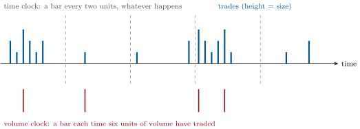
A strategy that does not trade on every message looks at the market through bars: summaries of the trades between two instants. The instants are chosen by a clock, and the clock need not be the wall clock.

Definition 2.1 (Bar, time bar, tick bar, volume bar, dollar bar, VWAP)

A bar summarises a run of consecutive trades by its open, high, low and close prices, its volume, its traded value and its number of trades. A time bar covers a fixed interval of wall-clock time; a tick bar a fixed number of trades; a volume bar closes on the trade at which its cumulative volume reaches a threshold, and a dollar bar on the trade at which its cumulative traded value does. The volume-weighted average price (VWAP) of a set of trades is $\sum_i p_iq_i/\sum_i q_i$ .

Definition 2.2 (Imbalance bar)

An imbalance bar closes when the absolute sum of the trade signs since its start, $|\theta| = |\sum b_i|$ , reaches a threshold set from the bars already closed: the expected number of trades per bar times the expected absolute imbalance per trade (López de Prado’s tick-imbalance bar), floored at the square root of the expected number of trades.

Figure 2.1. The same seventeen trades cut by two clocks. The time clock closes five equal intervals (dashed): three nearly empty, one holding the early burst and one the burst between

t = 6

and 7. The volume clock (solid, below) closes four bars: two short ones inside the bursts, ending at 0.7 and 6.9, and two long ones that absorb the quiet stretches; the last three trades wait for the next bar.

The floor is needed in practice. When buys and sells balance, the expected imbalance per trade is near zero and so is the threshold, and every trade would close a bar; the square root of $\E[T]$ is the level a random walk of signs first reaches after about $\E[T]$ trades.

Why sample by activity rather than by time? Because the variance of a price change grows with the amount of trading behind it, and trading is uneven.

Proposition 2.3 (Time bars are a variance mixture)

Suppose that, given the volume $V$ traded in a bar, the bar’s log return is $\mathcal N(0, \sigma^2V)$ . Then the kurtosis of time-bar returns is

\frac{\E[r^4]}{\E[r^2]^2} = \frac{3\,\E[V^2]}{\E[V]^2} = 3\bigl(1 + \mathrm{CV}(V)^2\bigr),

with $\mathrm{CV}$ the coefficient of variation of the bars’ volumes, while bars of equal volume have Gaussian returns.

Proof. $\E[r^2] = \sigma^2\E[V]$ and $\E[r^4] = 3\sigma^4\E[V^2]$ by conditioning on $V$ . A volume bar has $V$ constant, up to the last trade’s overshoot. ∎

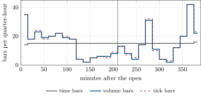
Clark (1973) proposed this subordination of prices to trading volume to explain heavy-tailed daily returns, and Ané and Geman (2000) found that returns sampled on a clock of trade counts were close to Gaussian. On the simulated day the one-minute bars’ volumes have a coefficient of variation of 0.94, so the proposition predicts a kurtosis of 5.67; the one-minute midquote returns have 5.44, and the close-to-close returns 5.47. The bars cut by the other clocks, with the same number of bars in the day (about 390), have kurtoses of 3.58 (tick), 4.04 (volume) and 3.92 (dollar): not 3, because in the simulator volatility follows the activity level and not volume exactly, but much closer. The event clocks spend their bars where the trading is (Figure 2.2): between 2 and 42 bars per quarter-hour, against a steady 15 for the time clock.

Figure 2.2. Bars closed per quarter-hour on the simulated day, each clock cutting about 390 bars. The time clock closes 15 bars in every quarter-hour; the volume and tick clocks follow the activity: busy after the open, quiet in the middle of the day, busy around the news burst at minute 210 (vertical line) and before the close. Dollar bars coincide with volume bars at this scale. Data: firm.tape, the chapter’s day, seeded.

2.3 What each representation destroys

Definition 2.4 (Midquote series)

A midquote series is the mid price $\tfrac12(b_t + a_t)$ sampled at chosen times, each value the last mid at or before the sampling time (an as-of sample).

A trade price is the mid plus or minus half the spread, depending on who initiated the trade. Sampled too finely, it bounces.

Proposition 2.5 (The bounce adds half a squared spread per return)

Let the trade price be $p = m + \tfrac s2 b$ , with a constant spread $s$ and trade signs $b = \pm1$ independent of each other and of the mid. Between two trades, $\E[(\Delta p)^2] = \E[(\Delta m)^2] + s^2/2$ .

Proof. $\Delta p = \Delta m + \tfrac s2(b_2 - b_1)$ , and $\E[(b_2 - b_1)^2] = 2$ when the signs are independent with mean zero. ∎

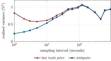
This is Roll’s model, whose estimator of the spread Book 4, chapter 21, derives; the same chapter’s signature plot draws the realised variance against the sampling interval. Here the plot answers the hook (Figure 2.3). At one second the trade-price variance of the day is 0.83 (in squared per cent) and the midquote’s 0.23; at five minutes they are 0.84 and 0.85. The trade price overstates at high frequency, as the proposition says. The midquote understates, for a reason the proposition does not see: in the simulator, as in real markets, the mid catches up with the efficient price in steps, a stale quote at a time, so its short-horizon returns are positively autocorrelated and their squares add up to less than the variance over longer horizons. Neither series is the efficient price.

Signature plot of the simulated day: realised variance of log returns against the sampling interval, from trade prices and from midquotes. At one second, 0.83 against 0.23; from about a minute on the two agree, and the noise of a single day’s estimate dominates. Data: firm.tape, the chapter’s day, seeded. — **Figure 2.3.** Signature plot of the simulated day: realised variance of log returns against the sampling interval, from trade prices and from midquotes. At one second, 0.83 against 0.23; from about a minute on the two agree, and the noise of a single day’s estimate dominates. Data: `firm.tape`, the chapter’s day, seeded.

The bounce is one loss among several, and a research store should know which each representation suffers:

Trade prices carry the bounce, and trades flagged with special conditions (odd lots, out-of-sequence reports, auction prints, late corrections: Book 1, chapter 28) mixed with regular ones. An opening auction print is a price at which a large volume traded at one instant; treating it as one more trade distorts the first bar of every day.
Midquotes cannot see what traded or how much, and at a wide spread the mid can move without any trade.
Bars lose the order of events inside the bar, the book, and every event between samples; the high and the low keep a trace of the path, which chapter 7’s range estimators exploit.
Time bars on several instruments are aligned in time but not in information: an illiquid instrument’s last trade may be minutes old (non-synchronous trading and the Epps effect, Book 4, chapter 21).
Any series stamped with one clock hides the difference between the exchange’s timestamp and the moment the data arrived; a backtest must use the second (chapter 3).

2.4 Continuous futures series

A futures contract expires, and its successor trades at a different price. A history long enough for research must splice contracts, and the splice is a choice.

Definition 2.6 (Continuous futures series, back-adjustment, ratio adjustment)

A continuous futures series follows the contract a position would hold under a roll rule: the nearby contract until a roll date some days before its last trading day, then the next contract. Back-adjustment adds, to every price before a roll, the gap between the new and the old contract on the roll date, so that the series has no jump at the roll and its latest prices are real. Ratio adjustment multiplies every earlier price by the ratio of the new contract’s price to the old one’s on the roll date instead.

Proposition 2.7 (What each adjustment preserves)

Ratio adjustment preserves the percentage returns of the rolled position on every day; back-adjustment preserves its price changes, the profit of one contract. Neither preserves the price levels of the past, and back-adjusted prices can be negative.

Proof. Between two roll dates both adjustments act on the held contract’s prices by a constant: an additive constant leaves differences unchanged, a multiplicative one leaves ratios unchanged. Across a roll date the adjustment is chosen so that the new contract’s price change (or return) is recorded, not the jump between contracts. Additive constants accumulate the roll gaps and can exceed a past price. ∎

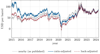
The crude oil futures settlements published by the US Energy Information Administration make the choice concrete (Figure 2.4). From 2 January 2015 to 5 April 2024 the nearby contract went from USD 52.69 to USD 86.91 a barrel, up 65%. A long position rolled five trading days before each of the 111 expiries of the period, the way a fund holding the nearby contract must, lost 27%: most of those years were in contango, and each roll sold a cheaper contract to buy a dearer one (the roll yield of One Quant Book 3, chapter 10). The ratio-adjusted series tells the fund’s story; its first price is USD 118.33. The back-adjusted series starts at USD 70.23 and, because the backwardation of 2021–2023 made the later gaps negative, reaches $-5.89$ on 21 April 2020, a day when the contract actually held (June 2020) settled at USD 11.57. The nearby series itself shows $-37.63$ on 20 April 2020, the settlement of an expiring contract no rolled position held.

WTI crude oil futures, 2015 to April 2024: the nearby contract as published (with -37.63 on 20 April 2020), and continuous series rolling five trading days before each expiry, ratio-adjusted (starting at 118.33) and back-adjusted (starting at 70.23, negative in April 2020). All three end at the same price. Data: US Energy Information Administration, NYMEX settlements, contracts 1 and 2. — **Figure 2.4.** WTI crude oil futures, 2015 to April 2024: the nearby contract as published (with $-37.63$ on 20 April 2020), and continuous series rolling five trading days before each expiry, ratio-adjusted (starting at 118.33) and back-adjusted (starting at 70.23, negative in April 2020). All three end at the same price. Data: US Energy Information Administration, NYMEX settlements, contracts 1 and 2.

Remark 2.8 (Which series for which question)

Returns of a rolled strategy: ratio-adjusted. Profit of a fixed number of contracts: back-adjusted differences. A signal on price levels (a moving average of the price, a breakout above a past high): neither without care, since both rewrite the past at every roll; compute the signal on the contract held at the time. The shape of the curve (carry, Book 8): the raw contracts, never an adjusted series.

2.5 Volumes, storage and formats

One simulated instrument-day of 1.56 million messages at 36 bytes (the size of an ITCH add-order message) is 56 MB before compression; the dated box shows what a whole exchange-day weighs. Three rules keep a research store usable.

Method 2.9 (Storing market data for research)

Keep the raw messages as received, immutable, with both timestamps, partitioned by date and instrument; every derived table (books, bars, features) is rebuilt from them by versioned code.
Store derived tables in a columnar, compressed format and partition them the way they are read: by date for cross-sectional work, by instrument for time-series work.
Record for every derived table the code version, the raw partitions it read and its parameters (the clock, the threshold, the roll rule), so that a result can name the exact data it used (chapter 29).

2.6 Tutorial: one day, four clocks

Goal. Simulate a trading day, cut it by four clocks and measure what each clock and each price does to the returns. End state: Figures 2.2 and 2.3; kurtoses 5.47 (time), 3.58 (tick), 4.04 (volume), 3.92 (dollar); the one-second variance ratio of 3.6.

The day. simulate(TapeConfig(seconds=23 400, u_shape=1.5, news_at=12 600, seed=3)) returns the messages, the trades, the top of book after every message and the efficient price (about 10 seconds).

Threshold bars. A bar closes on the trade that crosses the threshold; trades are never split between bars.

def _threshold_cuts(x, threshold: float):
    """Close a bar on the element at which the running sum of x reaches the threshold."""
    last, run = [], 0.0
    for i, v in enumerate(x):
        run += v
        if run >= threshold:
            last.append(i)
            run = 0.0
    last = np.array(last, dtype=int)
    first = np.concatenate([[0], last[:-1] + 1]) if len(last) else last
    return first, last


def tick_bars(t, px, qty, n: int) -> Bars:
    last = np.arange(n - 1, len(px), n)
    return _from_cuts(t, px, qty, last - n + 1, last)


def volume_bars(t, px, qty, threshold: float) -> Bars:
    first, last = _threshold_cuts(np.asarray(qty, float), threshold)
    return _from_cuts(t, px, qty, first, last)


def dollar_bars(t, px, qty, threshold: float) -> Bars:
    first, last = _threshold_cuts(np.asarray(px, float) * np.asarray(qty, float), threshold)
    return _from_cuts(t, px, qty, first, last)

Listing 2.1. Volume and dollar bars close on the crossing trade. code/firm/bars/firm_bars.py

Two prices, one day. Sample the last trade and the midquote on grids of 1 to 900 seconds and sum the squared log returns; compare the kurtosis with the mixture prediction from the bars’ volumes.

def realised_variance(tape, width: float) -> tuple[float, float]:
    """Realised variance of log returns on a grid of `width` seconds, from the last trade price and
    from the midquote at each grid time (units of 1e-4, i.e. squared percent)."""
    tt, m = mids(tape)
    tr = tape.trades
    g = np.arange(width, tape.cfg.seconds + 1e-9, width)
    rt = np.diff(np.log(asof(tr["t"], tr["price"], g)))
    rm = np.diff(np.log(asof(tt, m, g)))
    return float((rt**2).sum() * 1e4), float((rm**2).sum() * 1e4)


def clocks(tape, n_bars: int = 390):
    """Time, tick, volume and dollar bars, each with about n_bars bars over the day."""
    tr = tape.trades
    t, px, q = tr["t"], tr["price"] * tape.cfg.tick, tr["qty"].astype(float)
    return {
        "time": time_bars(t, px, q, tape.cfg.seconds / n_bars, 0.0, tape.cfg.seconds),
        "tick": tick_bars(t, px, q, len(t) // n_bars),
        "volume": volume_bars(t, px, q, q.sum() / n_bars),
        "dollar": dollar_bars(t, px, q, (px * q).sum() / n_bars),
    }


def mid_returns(tape, bars) -> np.ndarray:
    """Log midquote returns between bar ends (removes the bounce, keeps the clock)."""
    tt, m = mids(tape)
    return np.diff(np.log(asof(tt, m, bars.end)))


def mixture_kurtosis(volumes) -> float:
    """Kurtosis of a normal variance mixture whose variance is proportional to the bar's volume:
    3 E[V^2] / E[V]^2 = 3 (1 + CV^2)."""
    v = np.asarray(volumes, float)
    return 3.0 * float((v**2).mean() / v.mean() ** 2)

Listing 2.2. Realised variance from trades and from mids; the mixture kurtosis. code/research/02-market-data-for-research/python/rs_marketdata.py

Run summary() and fig_marketdata.py.

What to change next. Set act_vol=0 (no random activity) and watch the time bars’ kurtosis fall towards the mixture value of the U-shape alone; cut imbalance bars and follow their length through the day (exercise 7).

2.7 Build: the market simulator and the bar builders

Purpose. The book’s standard intraday data, with the truth attached: firm.tape writes an order-by-order feed from a known mechanism (efficient price, informed and noise flow, stale-quote cancellations); firm.bars turns trades into bars. Chapters 8–10 measure predictors on the tape, chapter 18 replays it, chapter 19 trades against it.

Interface. TapeConfig (duration, tick, levels, rates, Hawkes and metaorder parameters, efficient-price jump rate, news window, intraday profile, activity process, seed); simulate(cfg, v_path) returning a Tape of structured arrays msgs, trades (with true signs and an informed flag), top, and the paths v_t, v, act; simulate_pair(cfg, latency); Book().apply(msg). time_bars, tick_bars, volume_bars, dollar_bars, imbalance_bars, vwap, asof, continuous(c1, c2, expiry, days_before).

Rules. Deterministic for a seed. Rates piecewise constant between events except the Hawkes intensity, simulated exactly by thinning. The opening book is a snapshot at time zero. Prices are integer ticks, sizes integer shares.

Acceptance tests. code/firm/tape/tests/ and code/firm/bars/tests/: identical output for a seed; the messages rebuild the recorded top of book at every step and the book never crosses; executions equal trades; the mid tracks the efficient price; pooled over six seeds, imbalance predicts the next mid move and informed trades lose money for the resting side while noise trades pay it; bars close on the crossing trade; a hand-checked roll.

Stretch. Several instruments sharing a factor in their efficient prices; auctions at the open and close; a C++20 port of the event loop.

Sources and further reading

P. K. Clark, “A subordinated stochastic process model with finite variance for speculative prices”, Econometrica 41(1), 1973.
T. Ané and H. Geman, “Order flow, transaction clock, and normality of asset returns”, Journal of Finance 55(5), 2000.
D. Easley, M. López de Prado and M. O’Hara, “The volume clock: insights into the high-frequency paradigm”, Journal of Portfolio Management 39(1), 2012.
M. López de Prado, Advances in Financial Machine Learning, Wiley, 2018, chapter 2 (information-driven bars).
R. Roll, “A simple implicit measure of the effective bid–ask spread in an efficient market”, Journal of Finance 39(4), 1984.
Nasdaq, TotalView-ITCH 5.0 specification, and the sample files on emi.nasdaq.com.
US Energy Information Administration, NYMEX futures prices, crude oil contracts 1–4 (daily).

2.8 Exercises

Exercise 2.1 ★

Trades of 300 shares at 20.00, 500 at 20.02 and 200 at 19.99. What is their VWAP?

Solution

Solution of Exercise 2.1.

$(300 \times 20.00 + 500 \times 20.02 + 200 \times 19.99)/1\,000 = 20\,008/1\,000 = 20.008$ .

Exercise 2.2 ★

A stock at USD 20 has a one-cent spread and trades 20 000 times a day with a true daily volatility of 2%. By Proposition 2.5, what daily volatility does the sum of squared trade-to-trade log returns report?

Solution

Solution of Exercise 2.2.

The spread is $0.01/20 = 0.0005$ in log terms, so each trade-to-trade return gains $0.0005^2/2 = 1.25 \times 10^{-7}$ of variance; over 20 000 returns that is $0.0025$ . With the true $0.02^2 = 0.0004$ the sum is $0.0029$ : a reported volatility of 5.39%, 2.7 times the truth.

Exercise 2.3 ★

A feed averages 40 bytes a message and an active instrument 1.5 million messages a day. How much raw data do 5 000 such instruments produce in a year of 252 days?

Solution

Solution of Exercise 2.3.

$40 \times 1.5 \times 10^6 \times 5\,000 \times 252 = 7.56 \times 10^{13}$ bytes, about 76 terabytes a year before compression.

Exercise 2.4 ★★

One-minute volumes have a coefficient of variation of 0.8. What kurtosis does Proposition 2.3 predict for one-minute returns? What coefficient of variation gives a kurtosis of 6?

Solution

Solution of Exercise 2.4.

$3(1 + 0.8^2) = 4.92$ . A kurtosis of 6 needs $1 + \mathrm{CV}^2 = 2$ , a coefficient of variation of 1.

Exercise 2.5 ★★

A nearby contract settles at 70, 71, 72 on three days and the next contract at 73, 74, 76; the position rolls at the close of the second day. Give the held series, the back-adjusted and the ratio-adjusted series.

Solution

Solution of Exercise 2.5.

Held: 70, 71, 76 (the next contract from the third day). The roll gap on day two is $74 - 71 = 3$ . Back-adjusted: 73, 74, 76. Ratio-adjusted: $70 \times 74/71 = 72.96$ , $74$ , $76$ . The held position’s return on day three is $76/74 - 1 = 2.7\%$ , which the ratio-adjusted series shows and the raw nearby series ( $72/71$ then a jump) does not.

Exercise 2.6 ★★

A stock traded at USD 10 in 2015 and at USD 100 in 2025 with the same traded value every day. A volume-bar threshold fixed in shares gives how many bars a day in 2015 relative to 2025? And a dollar-bar threshold?

Solution

Solution of Exercise 2.6.

The same traded value is ten times as many shares at USD 10, so a threshold in shares closes ten times as many bars a day in 2015 as in 2025. Dollar bars close the same number in both years: value, not shares, measures the amount of trading.

Exercise 2.7 ★★★

Coding. Cut the chapter’s day into imbalance bars, starting from an expected 142 trades a bar. How many bars close, how many trades do they hold on average, and what is the kurtosis of their midquote returns? Why do the bars shrink through the day?

Solution

Solution of Exercise 2.7.

3 472 bars of 16.0 trades on average (the median bar has 7), with a midquote-return kurtosis of 35.4 (24.2 close to close). The threshold is re-estimated from the bars just closed. Because order signs are autocorrelated (metaorders), the imbalance reaches $\sqrt{\E[T]}$ in fewer than $\E[T]$ trades, the estimate of $\E[T]$ falls, and the threshold with it: the bars shrink until they close on short runs of one-sided flow, which is where large mid moves happen.

Exercise 2.8 ★★★

Find the flaw. “Our carry signal is the annualised log ratio of the back-adjusted second-month series to the back-adjusted front-month series, and our trend signal the percentage change of the back-adjusted front-month series over twelve months.”

Solution

Solution of Exercise 2.8.

Both signals use levels of a back-adjusted series, which are not prices: each has had later roll gaps added, so the ratio of two back-adjusted series is not the ratio of the two contracts’ prices (and a level can be negative, as in April 2020), and the twelve-month percentage change divides a dollar change by a fictitious base. Carry must be computed from the raw contracts on each date; the trend from ratio-adjusted returns (or from the back-adjusted change divided by the raw price held).

2.9 Problem: Which Clock?

Problem 2.1

Weekend problem — one day, four clocks and two prices

The chapter’s simulated day: 6.5 hours, a U-shaped profile, a random activity level and a news burst at 12 600 seconds, seed 3.

Part I — The feed.

How many messages and trades does the day have, and how many messages per trade?
What share of the messages are additions, cancellations and executions, roughly, and why are additions and cancellations nearly equal?
What is the raw size of the day at 36 bytes a message?
Why does a research store keep the messages rather than the bars?

Part II — Clocks.

How many bars does each clock cut, with thresholds chosen for about 390?
What are the kurtoses of close-to-close returns for the four clocks?
What is the coefficient of variation of the one-minute bars’ volumes, and what kurtosis does the mixture proposition predict for them?
Why are the event clocks’ kurtoses above 3?
Where in the day do volume bars concentrate, and why?

Part III — Prices.

What are the realised variances from trades and from mids at 1, 5, 60 and 300 seconds?
Which effect makes the trade series too high at one second?
Which makes the mid series too low?
From which interval on do the two agree within 5%?
What would you use to estimate the day’s variance from the one-second data (Book 4, chapter 21)?

Part IV — Judgement.

Which clock would you use for a daily volatility estimate, and which for a model of short-term price moves?
What does a one-minute time bar lose that a volume bar keeps?
What does a volume bar lose that a time bar keeps?
State the named result: the kurtosis of one-minute time-bar returns against dollar-bar returns on the day, and the trade-to-mid variance ratio at one second.
What in the simulator makes the time bars heavy-tailed, and what would remove it?
In one sentence: which representation is “the” price?

Solution

Solution of Problem 2.1.

1. 1 555 872 messages and 55 542 trades: 28.0 messages per trade. 2. Additions 49.3%, cancellations 47.2%, executions 3.6%: almost every order added is later cancelled, since market orders remove only a small share of the resting volume. 3. $1\,555\,872 \times 36 = 56.0$ MB. 4. Every coarser view can be rebuilt from them, and bars fixed today would freeze a clock, a threshold and a price choice into every later study. 5. Time 390, tick 391, volume 388, dollar 388. 6. 5.47, 3.58, 4.04 and 3.92. 7. 0.94; $3(1 + 0.94^2) = 5.67$ , against 5.47 measured. 8. Volatility follows the activity level, not volume exactly (and the news burst moves the efficient price faster for a given volume), so equal-volume bars still mix variances. 9. After the open, around the news burst and before the close, where the activity multiplier and the U-shape put the trading. 10. Trades 0.83, 0.58, 0.96, 0.84; mids 0.23, 0.39, 0.93, 0.85 (squared per cent). 11. The bid–ask bounce (Proposition 2.5). 12. The mid adjusts to the efficient price in steps, so its short-horizon returns are positively autocorrelated. 13. From about 45 seconds on (0.95 against 0.91, then within 3.4%). 14. A noise-robust estimator on the one-second data: two-scales realised variance, the realised kernel or pre-averaging. 15. Time bars at five minutes or more (or a noise-robust estimator) for the day’s variance; an event clock, or the messages themselves, for short-term moves. 16. Nothing of the activity: it keeps a regular calendar, aligned across instruments, but its returns mix quiet and busy periods. 17. A common calendar: its bars end at different times on different instruments and on different days. 18. Named result: the one-minute time bars have a kurtosis of 5.47 and the dollar bars 3.92, and at one second the trade-price variance is 3.6 times the midquote’s. 19. The random activity level that scales both volume and the efficient price’s speed; with act_vol=0 only the U-shape and the news burst remain. 20. None: the efficient price is unobserved, and trades, mids and bars are noisy views of it, each with its own error.

2.10 Interview questions

Interview question 2.1 ★ researcher, trader

Why might you sample prices by volume rather than by time?

Solution

Solution of Interview question 2.1.

Because price variance accumulates with trading, not with time; bars of equal volume (or value) have returns much closer to Gaussian and less heteroskedastic, which helps statistics that assume both. The cost: bars no longer align in time across instruments, and the clock itself reacts to news.

What the interviewer is looking for: subordination to volume; the loss of a common calendar.

Interview question 2.2 ★★ researcher

Your realised volatility from one-second trade prices is double the one from five-minute prices. What is going on?

Solution

Solution of Interview question 2.2.

Microstructure noise: the bid–ask bounce adds about $s^2/2$ per return, which dominates at high frequency. The signature plot shows it; fixes are sampling less often, using midquotes, or a noise-robust estimator.

What the interviewer is looking for: the bounce, the signature plot, and a fix.

Interview question 2.3 ★★ researcher, trader

How would you build a continuous futures series for a trend-following backtest, and what goes wrong with back-adjusted prices?

Solution

Solution of Interview question 2.3.

Roll on a rule a real position would follow (a fixed number of days before expiry, or on open interest); compute returns from the held contract (ratio-adjusted), and signals on levels from the contract held at the time. Back-adjusted levels rewrite the past at every roll and can go negative; percentage changes of them are wrong.

What the interviewer is looking for: returns versus levels, and that the adjustment is a modelling choice.

Interview question 2.4 ★★ developer, researcher

Design the storage of a year of order-by-order data for 5 000 instruments for research use.

Solution

Solution of Interview question 2.4.

Raw messages immutable, with exchange and receive timestamps and sequence numbers, partitioned by date and instrument, compressed; about 76 TB a year raw at 40 bytes and 1.5 million messages per instrument-day. Derived tables (books, bars) rebuilt by versioned code, stored columnar, partitioned the way they are read, each with its lineage recorded.

What the interviewer is looking for: immutability, lineage, the partitioning, and an order-of-magnitude size.

Interview question 2.5 ★★ researcher, mle

A colleague’s model uses one-minute bars of fifty stocks. What can go wrong because the bars are time bars?

Solution

Solution of Interview question 2.5.

Non-synchronous closes: the last trade of an illiquid stock may be minutes old, which creates spurious lead–lag and shrinks correlations (the Epps effect); the bounce in close prices; heteroskedasticity from uneven activity; auction prints in the first and last bars.

What the interviewer is looking for: non-synchronicity and noise, not only look-ahead.

Interview question 2.6 ★★★ researcher

Show that if returns are normal given the volume traded, time-bar returns have kurtosis $3(1 + \mathrm{CV}^2)$ .

Solution

Solution of Interview question 2.6.

Given $V$ , $r \sim \mathcal N(0, \sigma^2V)$ , so $\E[r^2] = \sigma^2\E[V]$ and $\E[r^4] = 3\sigma^4\E[V^2]$ ; the ratio is $3\E[V^2]/\E[V]^2 = 3(1 + \mathrm{CV}^2)$ .

What the interviewer is looking for: conditioning on the volume and the fourth moment of a normal.

Terms defined in this chapter

See all 2333 terms in the glossary