Research Craft: Predictors, Backtests, Measurement, Portfolios · Research
13Half-Life, Decay and Stability
McLean and Pontiff (2016) followed 97 variables that published studies had shown to predict the cross-section of stock returns, past the samples of the studies and past their publication. Portfolio returns were 26% lower out of sample and 58% lower after publication; they read the difference, 32%, as the effect of investors trading on what they had read. Every signal a desk owns is on some such path, and the questions of this chapter are how fast a predictor’s information runs out as the horizon lengthens, how stable it is from year to year, and how to tell a predictor that has died from one that was unlucky. The clock of the first question is days; of the second, years; the third is a problem of statistical power, and its answer is often that the data cannot tell.
13.1 Decay across horizons
Definition 13.1 (IC decay curve, signal autocorrelation, signal half-life)
The IC decay curve of a predictor is its information coefficient with the return of the single period , as a function of the lag . The signal autocorrelation is the cross-sectional rank correlation of the predictor with itself periods earlier, averaged over dates. The signal half-life is the lag at which it falls to one half; for a first-order autoregression with coefficient per period it is (the half-life of Book 4, chapter 4).
The two curves answer different questions. The IC decay curve says how long the information lasts, and so the holding period; the signal autocorrelation says how fast the predictor itself changes, and so the turnover. A rank-weighted book rebuilt every period trades a fraction of about of itself, where is the lag-one signal autocorrelation. On firm.synthmkt (Figure 13.1 and the table), four predictors show four shapes:
| predictor | IC, | curve half-life | autocorr. | signal half-life | turnover |
|---|---|---|---|---|---|
| reversal, 1 day | 0.037 | 1 day | — | 104% | |
| surprise, 60 days | 0.010 | 20 days (fit) | 0.983 | 39 days | 1.7% |
| momentum 12-1 | 0.008 | none in 60 days | 0.995 | 130 days | 0.53% |
| book-to-price | 0.004 | none in 60 days | 0.9995 | 1 386 days | 0.05% |
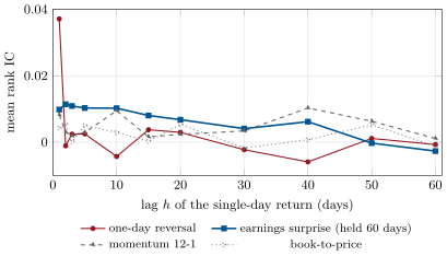
firm.synthmkt: the rank IC of each predictor known at the close of day with the return of day alone, averaged over eight years of dates. Reversal lives one day; the surprise’s planted 60-day drift falls to zero at 60 days; momentum and value are too slow to decay within the window.The table carries two warnings. The surprise’s curve is not exponential: every event drifts at a constant rate for 60 days, and a signal observed at a random age has a remaining drift that falls linearly to zero, so the curve is a straight line with a kink; an exponential fit reports a half-life of 20 days for a planted life of 60. Fitting a form assumes it. And the slow predictors’ daily ICs, 0.004 to 0.008, are close to their sampling noise; their decay cannot be measured on single days, only on longer returns and many years. The practical reading is on the turnover column: the one-day reversal trades its whole book every day and pays costs to match (chapter 27), book-to-price a twentieth of a percent.
13.2 Stability across years
Definition 13.2 (IC stability)
The IC stability of a predictor is the behaviour of its information coefficient across non-overlapping periods: the dispersion of yearly (or monthly) ICs around their mean, compared with the dispersion their sampling error alone would produce.
The monthly IC of a signal is a noisy number, and its noise is not only sampling error in the cross-section: when the predictor loads on a common factor, the factor’s return that month moves every stock’s return together and with it the IC. Momentum on the synthetic market (planted constant for ten years) has a mean monthly IC of 0.023 and a standard deviation of 0.247; its yearly means run from to 0.18, and a block-bootstrap 95% interval for the mean runs from to 0.071, across zero. The earnings surprise has a mean of 0.040 with a standard deviation of 0.041, and its yearly means stay between 0.02 and 0.06. Two constant predictors, one of which looks stable and one of which looks like a sequence of regimes: the difference is the factor exposure, not the truth.
13.3 Structural breaks
Definition 13.3 (Structural break, CUSUM test)
A structural break is a change, at some date, in the parameters of the process generating a series (here, the mean of a predictor’s IC). The CUSUM test of Brown, Durbin and Evans (1975) cumulates the standardised recursive residuals (each observation minus the mean of those before it, rescaled) and rejects constancy when the path leaves a pair of lines that widen linearly with time, with at 5% for residuals.
The alternative is to try every date: fit one mean before and one after, compute the F statistic of the split, and take the largest over the middle of the sample (Andrews, 1993, gave the theory of this sup-F statistic for a change at an unknown point; Bai and Perron, 1998, extended it to several breaks). firm.decay computes its p-value by permutation, which keeps the series’ own distribution (heavy tails included) and assumes only that, without a break, the order of the months is irrelevant.
A planted break makes the comparison. With pead_break at the start of year 7, the synthetic market’s post-earnings drift is removed entirely: the surprise’s mean monthly IC falls from 0.032 before to 0.005 after (Figure 13.2). The sup-F statistic, 12.5, peaks 53 months into the series (the break is at 48, and old announcements keep drifting for up to 60 days after it), with a permutation p-value of 0.013. The CUSUM does not cross its boundary: its path reaches 0.69 of it. With the drift cut by 70% instead of removed, neither test sees anything in this market (sup-F p-value 0.93). One market is one draw; over ten markets with different seeds, sup-F detects the removal in all ten, the 70% cut in seven and a change that never happened in one, the CUSUM in five, three and one. And momentum, which nothing changed, fails both: its CUSUM crosses in the last month, its sup-F p-value is 0.023, after a few strong years. A 5% test rejects a stable predictor one time in twenty by design, more often when the IC’s variance changes over time, and a desk that monitors fifty predictors monthly will see breaks every year that are not there.
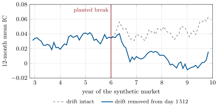
firm.synthmkt, with the post-earnings drift intact and with it removed from the start of year 7 (day 1 512). The sup-F test finds the break (p-value 0.013); the CUSUM does not; in this market a 70% cut is found by neither.13.4 Post-publication decay
Definition 13.4 (Post-publication decay)
The post-publication decay of a predictor is the fall of its return, or its IC, after the study that documented it was published, relative to the period the study could have examined.
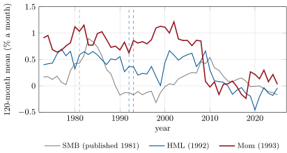
Three of the most studied factors show it in the Kenneth French data library (the chapter stores only derived statistics). Taking each from July 1963 to the end of the year its paper appeared (Banz, 1981, for size; Fama and French, 1992, for value; Jegadeesh and Titman, 1993, for momentum) and from then to July 2026:
| factor (paper) | mean a month, before | mean a month, after | decline | ||
|---|---|---|---|---|---|
| SMB (1981) | 0.47% | 2.25 | 0.01% | 0.10 | 97% |
| HML (1992) | 0.42% | 3.12 | 0.19% | 1.16 | 55% |
| Mom (1993) | 0.85% | 4.76 | 0.37% | 1.54 | 56% |
The declines bracket McLean and Pontiff’s average, and the rolling ten-year means show them (Figure 13.3). Yet a sup-F test for one break over the whole monthly history from 1963 rejects for none of the three at 5% (permutation p-values 0.18, 0.15 and 0.053). Factor returns are noisy enough that a halving over decades is hard to date statistically, and a publication date is only one of many candidate causes: Chordia, Subrahmanyam and Tong (2014) found that the returns of a portfolio of prominent anomalies roughly halved after decimalisation, with hedge-fund assets, short interest and turnover behind the decline. A replication adds a third reading: Hou, Xue and Zhang (2020) found that 65% of 452 anomalies could not clear a statistic of 1.96 once microcaps were mitigated, and that even the replicated ones were much smaller than originally reported. Some of the decay is the original sample’s selection.
13.5 Measuring the half-life of a predictor card
Every predictor card (chapter 6) carries a horizon and half-life field, and this chapter’s tools fill it: the IC decay curve at the card’s sampling frequency, its fitted half-life with a bootstrap interval (and the warning of the surprise: plot the curve before trusting the form), the signal autocorrelation and the turnover it implies, and the monthly IC series with its CUSUM and sup-F tests, refreshed every month. The hardest question is the last one: when the recent IC is half the historical one, is the predictor dying? Two periods of months each with a monthly IC of mean and standard deviation give two means with standard error ; the probability of measuring a halving when nothing changed and when the IC truly halved depends only on the statistic of a period.
Proposition 13.5 (The evidence of a measured halving)
With prior probability that the IC truly halved, a measured halving (second-period mean at most half the first) has posterior probability of true decay, where and are the probabilities of the measurement without and with decay; for normal means is close to and falls with the period’s statistic.
Proof. Bayes’ rule on the two hypotheses. With decay, the second mean is centred on half the first’s centre with the same noise, and the event “second at most half the first” is nearly symmetric about that centre, so ; without decay the event needs the noise to move the means apart by half their level, whose probability falls as the level grows against the noise. ∎
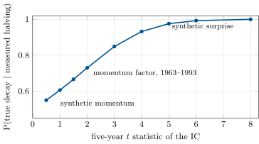
With and five-year periods (Figure 13.4), a predictor with the synthetic momentum’s noise (a five-year statistic of 0.72) that measures a halving has truly decayed with probability 0.57, barely more than the prior; one with the momentum factor’s pre-publication noise (), 0.72; one as steady as the synthetic surprise (), 0.999. A decline is evidence in proportion to the predictor’s precision; for noisy predictors, the decision to cut must rest on other evidence (capacity, crowding, the mechanism) or on longer samples.
13.6 Tutorial: dating a predictor’s decline
Goal. Measure the decay curves and half-lives of four synthetic predictors, test a planted break with the CUSUM and sup-F tests, measure three real factors before and after publication, and compute the evidence a measured halving carries. End state: Figures 13.1, 13.2, 13.3 and 13.4; the two tables.
Fit the curve by least squares over a grid of half-lives, negative ICs included.
def half_life_fit(horizons, ic, grid=None) -> tuple[float, float]:
    """Least squares over all horizons (negative ICs included): for each half-life on a log grid the best ic0 is
    closed-form; returns the pair with the smallest squared error (the grid's top end means 'no visible decay')."""
    h, y = np.asarray(horizons, float), np.asarray(ic, float)
    grid = np.geomspace(0.1, 2000.0, 800) if grid is None else np.asarray(grid, float)
    best = (np.inf, 0.0, 0.0)
    for hl in grid:
        g = 2.0 ** (-h / hl)
        ic0 = float(g @ y / (g @ g))
        sse = float(np.sum((y - ic0 * g) ** 2))
        if sse < best[0]:
            best = (sse, ic0, float(hl))
    return best[1], best[2]
Listing 13.1. Least-squares half-life of an IC decay curve. code/firm/decay/firm_decay.py The CUSUM path and its boundary.
def cusum(x) -> tuple[np.ndarray, np.ndarray]:
    """Recursive residuals of a constant-mean model, w_t = (x_t - mean of x_1..x_{t-1}) * sqrt((t-1)/t), scaled by
    their standard deviation and cumulated; the 5% boundary is +/- 0.948 (sqrt(K) + 2 (t - k) / sqrt(K)), K the
    number of recursive residuals (Brown, Durbin and Evans)."""
    x = np.asarray(x, float)
    t = np.arange(1, len(x))
    prev_mean = np.cumsum(x)[:-1] / t
    w = (x[1:] - prev_mean) * np.sqrt(t / (t + 1.0))
    W = np.cumsum(w) / w.std(ddof=1)
    K = len(w)
    b = 0.948 * (np.sqrt(K) + 2.0 * np.arange(1, K + 1) / np.sqrt(K))
    return W, b
Listing 13.2. Brown, Durbin and Evans’s CUSUM for a constant mean. code/firm/decay/firm_decay.py - Run
decay_table(),stability()with and without the planted break,factors(),power()andfig_decay.py;rs_fetch_factors.pyonce for the French statistics.
What to change next. Plant a gradual decay instead of a break (a drift that falls linearly over three years) and see which test finds it first; repeat the post-publication table with the sample of each paper instead of 1963.
13.7 Build: the decay toolkit
Purpose. The horizon, half-life and stability fields of every predictor card, measured the same way, and monthly monitoring of the predictors in production.
Interface. ic_decay(signal, ret, horizons, dates), half_life_fit, rank_autocorr, half_life_ar, turnover, block_bootstrap, cusum, sup_f, sup_f_critical, sup_f_pvalue, decline_power(ic, sd, n, ratio); firm.synthmkt gains pead_break and pead_after (off by default).
Rules. A decay curve uses single-period returns at each lag, never cumulative ones; every half-life is reported with the form it assumes; a break test’s p-value comes with the number of predictors monitored.
Acceptance tests. code/firm/decay/tests/: a planted five-day signal half-life recovered by the curve fit and the autocorrelation; a one-day signal; bootstrap shape; CUSUM silent on noise and crossing on a planted shift; sup-F locating the shift, its simulated critical value, permutation p-values on a shift, on noise and on heavy-tailed noise; the power probabilities.
Stretch. Bai–Perron for several breaks; a Bayesian change-point model with a prior on decay; decay curves by capacity bucket.
Sources and further reading
- R. D. McLean and J. Pontiff, “Does academic research destroy stock return predictability?”, Journal of Finance 71(1), 2016.
- T. Chordia, A. Subrahmanyam and Q. Tong, “Have capital market anomalies attenuated in the recent era of high liquidity and trading activity?”, Journal of Accounting and Economics 58(1), 2014.
- K. Hou, C. Xue and L. Zhang, “Replicating anomalies”, Review of Financial Studies 33(5), 2020.
- R. L. Brown, J. Durbin and J. M. Evans, “Techniques for testing the constancy of regression relationships over time”, Journal of the Royal Statistical Society B 37(2), 1975.
- D. W. K. Andrews, “Tests for parameter instability and structural change with unknown change point”, Econometrica 61(4), 1993; J. Bai and P. Perron, “Estimating and testing linear models with multiple structural changes”, Econometrica 66(1), 1998.
- R. W. Banz, Journal of Financial Economics 9(1), 1981; E. F. Fama and K. R. French, Journal of Finance 47(2), 1992; N. Jegadeesh and S. Titman, Journal of Finance 48(1), 1993; Kenneth R. French Data Library.
13.8 Exercises
Exercise 13.1 ★
A signal’s lag-one daily rank autocorrelation is 0.98. What are its half-life and the daily turnover of a book that holds it?
Solution
Solution of Exercise 13.1.
days; a rank-weighted book trades about of itself a day.
Exercise 13.2 ★
A factor earned 0.85% a month before publication and 0.37% after. What is the decline, and how does it compare with McLean and Pontiff’s average?
Solution
Solution of Exercise 13.2.
(56.0% on the unrounded means), close to McLean and Pontiff’s average post-publication decline of 58%.
Exercise 13.3 ★
With recursive residuals, where is the CUSUM’s 5% boundary at the first residual and at the last?
Solution
Solution of Exercise 13.3.
at the first residual and at the last.
Exercise 13.4 ★★
Every event drifts at a constant rate for 60 days after its announcement and the signal is observed at a uniformly random age between 0 and 59 days. Show that the share of signals still drifting on day is , and explain why the IC decay curve then falls linearly to zero at 60 days rather than halving at a fixed rate.
Solution
Solution of Exercise 13.4.
A signal of age still drifts on day if , which for uniform on has probability . The single-day IC at lag is proportional to the share of signals still drifting (each drifts at the same rate), so it falls linearly and reaches zero at . An exponential has no end and a constant halving time; forced onto a straight line that stops, it reports a half-life that describes neither the start nor the end.
Exercise 13.5 ★★
A monthly IC has mean 0.04 and standard deviation 0.10. What is the five-year statistic, and roughly what posterior of true decay does a measured halving give, with a prior of one half?
Solution
Solution of Exercise 13.5.
. By the curve of Figure 13.4, a measured halving then has a posterior of about 0.86 (rs_decay.power(0.04, 0.10) gives 0.858).
Exercise 13.6 ★★
Why does a predictor that loads on a common factor have a noisier monthly IC than one that does not, even with the same true information?
Solution
Solution of Exercise 13.6.
Each month the factor’s realised return moves all loaded stocks together, in the direction of the predictor’s ranks or against them; the rank correlation with returns then swings with the factor, whatever the predictor’s stock-specific information. The swings are common to the whole cross-section, so they do not average out over stocks, only over months.
Exercise 13.7 ★★★
Coding. With rs_decay.detection, measure how often sup-F and the CUSUM detect a 50% cut of the drift at year 7 over the ten seeds, and place it between the chapter’s removal and 70% cut.
Solution
Solution of Exercise 13.7.
rs_decay.detection(0.5): sup-F detects a 50% cut in three markets of ten and the CUSUM in one, between the 70% cut (seven and three) and no change at all (one and one, the false alarms). Over a ten-year market with four years after the break, halving a predictor’s drift is found less often than not.
Exercise 13.8 ★★★
Find the flaw. “Our momentum signal’s IC over the last 24 months is a third of its 10-year average and the CUSUM crossed its boundary last month; we are switching it off.”
Solution
Solution of Exercise 13.8.
A 24-month IC of momentum is dominated by the factor’s realised returns: on the synthetic market the monthly IC has a standard deviation of 0.25 against a mean of 0.02, so two years say almost nothing (a halving is barely evidence at a five-year of 0.72, and a third over two years even less). The CUSUM crossing in the last month is exactly what the synthetic momentum did with nothing changed. Before switching off: the test’s false-alarm rate across all monitored predictors, the mechanism, crowding and capacity evidence (chapter 28), and a longer sample.
13.9 Problem: Did It Die, or Was It Unlucky?
Problem 13.1
Weekend problem — a decline, weighed
The chapter’s four synthetic predictors, the surprise with its drift removed at year 7, and the French factors.
Part I — Horizons.
- Give the one-day IC and the signal autocorrelation of each predictor.
- Why does the reversal’s book turn over completely each day?
- What half-life does an exponential fit give the surprise, and what is its planted life?
- Why can momentum’s and value’s decay not be measured on single days?
Part II — Years.
- Give the mean and standard deviation of the monthly IC for momentum and for the surprise.
- What is the bootstrap interval for momentum’s mean IC?
- Why is momentum’s IC so much noisier?
- What do the CUSUM and sup-F tests say about momentum, which the simulator holds constant?
Part III — Breaks.
- What are the surprise’s mean IC before and after the planted removal?
- Where does sup-F put the break, with what statistic and p-value? Why not exactly at month 48?
- What does the CUSUM find?
- What happens with a 70% cut instead, in this market and over ten markets?
- Give the three factors’ declines after publication and the sup-F p-values over their whole histories.
Part IV — The verdict.
- What are and for a predictor with the synthetic momentum’s noise?
- State the named result: the probability that a signal whose measured IC halved over five years has truly decayed, for the three precisions of the chapter.
- What statistic makes a measured halving 90% convincing?
- What other evidence would you seek before switching off a noisy predictor?
- How would you set a monitoring rule for fifty predictors so that false alarms stay rare?
- Which readings besides investors’ trading can explain a post-publication decline?
- In one sentence: when is a decline evidence?
Solution
Solution of Problem 13.1.
- Reversal 0.037 and ; surprise 0.010 and 0.983; momentum 0.008 and 0.995; book-to-price 0.004 and 0.9995.
- Its signal is today’s return, uncorrelated with yesterday’s (): the ranks are new every day, and a book that follows them is rebuilt every day (turnover ).
- 20 days; the planted drift lasts 60 days.
- Their single-day ICs (0.004 to 0.008) are near their sampling noise, and a half-life of months cannot show within 60 days.
- Momentum: mean 0.023, standard deviation 0.247. Surprise: 0.040 and 0.041.
- From to 0.071.
- It loads on the momentum factor, whose monthly return moves the whole cross-section.
- Both reject at 5%: the CUSUM crosses in the last month, and sup-F has a permutation p-value of 0.023, with nothing changed.
- 0.032 before and 0.005 after.
- At month 53, statistic 12.5, p-value 0.013. Old announcements keep drifting for up to 60 days after the break, so the IC falls over three months.
- Nothing: its path reaches 0.69 of the boundary.
- In this market neither test sees it (sup-F p-value 0.93); over ten markets sup-F detects it in seven and the CUSUM in three.
- SMB 97%, HML 55%, Mom 56%; sup-F p-values 0.18, 0.15 and 0.053.
- and .
- Named result. With a prior of one half, a measured halving over five years means true decay with probability 0.57 for a predictor with the synthetic momentum’s noise (), 0.72 with the momentum factor’s pre-publication noise (), and 0.999 for one as steady as the synthetic surprise ().
- About 3.6: with the posterior is , which reaches 0.9 when , that is (Interview question 6), .
- The mechanism (is there a reason it should have stopped?), crowding and capacity measures, the predictor’s correlation with newly published ones, trading costs, and the same predictor’s behaviour in other markets.
- Control the false alarms across predictors (a stricter level, or a false-discovery rate, chapter 20), require persistence (two consecutive alarms), and act on size before switching off: reduce the weight when the evidence is weak, remove when it is strong.
- The original sample’s selection (a false or overstated discovery regresses), changes in market structure (decimalisation, liquidity, costs), and risk that was priced and is priced less. McLean and Pontiff separate the first from trading by comparing out-of-sample and post-publication periods.
- When the predictor is precise enough that a decline of that size would rarely happen by chance.
13.10 Interview questions
Interview question 13.1 ★ researcher
What is the half-life of a signal, and how does it relate to turnover?
Solution
Solution of Interview question 13.1.
The lag at which the signal’s autocorrelation falls to one half, for a lag-one autocorrelation . A book that tracks the signal trades about of itself each period, so short half-lives mean high turnover and costs; the information’s own half-life, from the IC decay curve, sets the holding period, and the two need not agree.
Interview question 13.2 ★★ researcher
How would you measure how fast a predictor’s information decays with horizon?
Solution
Solution of Interview question 13.2.
Compute its IC with the return of each single future period (not cumulative returns, which mix horizons), average over many dates, and plot against ; fit a form only after looking at the curve, with bootstrap intervals over dates.
Interview question 13.3 ★★ researcher, trader
Your best signal has had a bad year. How do you decide whether it is broken?
Solution
Solution of Interview question 13.3.
Compare the year with the IC’s own noise: its statistic per year, the probability of such a year with nothing changed, and a break test with a p-value that accounts for heavy tails (permutation) and for the number of signals monitored. Then look for other evidence: mechanism, crowding, capacity. A single bad year of a noisy signal is weak evidence.
Interview question 13.4 ★★ researcher
Why do anomalies weaken after publication? Give three explanations and a way to tell them apart.
Solution
Solution of Interview question 13.4.
Statistical bias in the original discovery (it regresses out of sample), investors trading on the publication, and changes in market structure or costs unrelated to publication. McLean and Pontiff tell the first two apart with the out-of-sample but pre-publication period (a 26% decline, an upper bound on data mining) against the post-publication period (58%); dating the decline against structural changes (decimalisation) tests the third.
Interview question 13.5 ★★ researcher
Compare the CUSUM and sup-F tests for a change in a signal’s mean.
Solution
Solution of Interview question 13.5.
The CUSUM cumulates standardised recursive residuals and rejects when the path leaves boundaries that widen with time; it needs no candidate date and is cheap, but on this chapter’s planted removal it did not cross. Sup-F tries every date, is powerful against a single shift in the mean, and locates it; its critical value must account for the search (Andrews) or be computed by permutation. Both are one-break tests of the mean and both reject stable noisy series at their nominal rate.
Interview question 13.6 ★★★ researcher
Derive the probability that a signal’s second five-year mean IC is at most half its first when nothing has changed, as a function of the IC’s statistic.
Solution
Solution of Interview question 13.6.
Let the two means be and with and independent standard normals. The event is , and is normal with variance , so the probability is with : 0.37 at , 0.19 at , 0.0004 at .