Research Craft: Predictors, Backtests, Measurement, Portfolios · Research

20Overfitting

A thousand parameter settings of a moving-average trend system are backtested on eighteen years of daily returns. The best has a Sharpe ratio of 0.44; over the next five years it loses, with a Sharpe ratio of $-0.32$ . The returns were pure noise, and the thousand systems a search through it. Run the same search on returns with a real, planted trend and the best system in the search years again disappoints afterwards, earning less than the average system: the trend was there for all of them, and the search picked noise on top of it. Overfitting in finance is rarely a model with too many parameters; it is a choice among too many backtests, measured on too little history. This chapter measures it (the probability of backtest overfitting), bounds it (the minimum backtest length), and prevents the leak that makes it invisible in cross-validation (purging and embargo), with firm.overfit.

20.1 Selection under many trials

Definition 20.1 (Backtest overfitting, in-sample, out-of-sample)

In-sample data are those used to build or choose a strategy; out-of-sample data are those it has not seen. Backtest overfitting is the selection of a strategy whose in-sample performance owes more to the particular sample than to a property that persists, so that its out-of-sample performance falls short of what was selected.

The chapter’s systems hold the market long when a fast moving average of the price is above a slow one, short otherwise: fast windows of 2 to 40 days, slow windows of 50 to 540, a thousand pairs. On 25 years of synthetic daily returns, the first 20 are the search (17.9 years once the longest average has started), the last five the test. On pure noise the best system’s in-sample Sharpe ratio is 0.44, its out-of-sample $-0.32$ ; the median system’s in-sample 0.17. The expected best of a thousand independent null strategies over 17.9 years would be 0.77 (Book 4, chapter 12); the systems are far from independent (their Sharpe ratios have a standard deviation of only 0.076 around a common level), and the maximum expected from that dispersion is 0.25 above the common level, about what was found.

With a planted trend, a persistent drift of the kind trend-followers earn (a half-life of 120 days), every system earns it: the median in-sample Sharpe ratio is 0.50, the average out-of-sample 0.26. The best in-sample system, 0.77, earns 0.14 out of sample, less than the average system. The ranking is not useless (across the systems, in-sample and out-of-sample Sharpe ratios correlate at 0.33, and the fifty best in sample earn 0.29 out of sample), but the single winner is where the noise concentrates: the search found the trend, and choosing one point of it paid for noise. On noise the correlation is $-0.05$ and the fifty best earn $-0.02$ .

20.2 The probability of backtest overfitting

Definition 20.2 (Probability of backtest overfitting, combinatorially symmetric cross-validation)

The probability of backtest overfitting (PBO) of a selection procedure is the probability that the strategy it selects as the best in sample performs below the median of the candidates out of sample. Combinatorially symmetric cross-validation (CSCV) estimates it by cutting the history into $S$ blocks and, for each choice of $S/2$ blocks as the in-sample set, ranking the in-sample winner among all candidates on the other half; the PBO is the share of splits where its rank is below the median (Bailey, Borwein, López de Prado and Zhu).

The rank $\omega$ of the winner among $N$ candidates, as a fraction, is turned into a logit $\lambda = \ln(\omega/(1 - \omega))$ : positive when the winner stays above the median, negative when it falls below. With 16 blocks there are 12 870 splits; firm.overfit.cscv uses 3 000 of them, drawn at random, and computes every split’s Sharpe ratios as matrix products of block sums. The PBO of the thousand-system search is 0.82 on noise and 0.74 with the planted trend (Figure 20.1); the regression of the winners’ out-of-sample Sharpe ratios on their in-sample ones has slopes of $-0.89$ and $-0.91$ . A PBO above one half means selection is worse than choosing at random: among correlated systems, the in-sample winner is the one that fitted the noise of its half best, and the noise of the other half is its mirror.

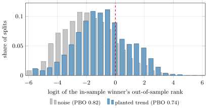
Figure 20.1. CSCV on the thousand trend systems’ search years (16 blocks, 3 000 splits): the distribution of the logit of the in-sample winner’s out-of-sample rank. Mass to the left of zero is the probability of backtest overfitting. Data: rs_overfit on synthetic returns.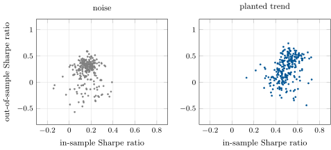

In-sample (17.9 years) against out-of-sample (5 years) Sharpe ratios of the trend systems (every fourth of the thousand). On noise the clouds are unrelated (correlation -0.05); with the trend they correlate at 0.33, yet the top in-sample system is not near the top out of sample. Data: rs_overfit.systems. — **Figure 20.2.** In-sample (17.9 years) against out-of-sample (5 years) Sharpe ratios of the trend systems (every fourth of the thousand). On noise the clouds are unrelated (correlation $-0.05$ ); with the trend they correlate at 0.33, yet the top in-sample system is not near the top out of sample. Data: `rs_overfit.systems`.

20.3 Minimum backtest length

Definition 20.3 (Minimum backtest length)

The minimum backtest length for $N$ trials and a target Sharpe ratio is the number of years of history below which the expected best of $N$ strategies with no skill has an in-sample Sharpe ratio at or above the target.

Proposition 20.4 (How much history a search needs)

If $N$ independent strategies with no skill are each measured over $y$ years, their annual Sharpe ratio estimates have variance about $1/y$ , and the expected maximum grows like $\sqrt{2\ln N/y}$ ; a target Sharpe ratio $s$ is expected to be reached by chance unless $y \gtrsim 2\ln N/s^2$ .

Proof. The expected maximum of $N$ standard normals grows like $\sqrt{2\ln N}$ (Book 4, chapter 12); scale by the standard error $1/\sqrt y$ and solve $\sqrt{2\ln N/y} = s$ . ∎

With the expected maximum computed exactly (firm.multitest.expected_max_sr), a thousand trials need 10.6 years before a Sharpe ratio of 1 stops being expected from luck, 42.4 years for 0.5, and 3.3 years for 1.8 (Figure 20.3). The bound is conservative when the trials are correlated, as the trend systems are, and a guide when they are not; its lesson is the scaling: four times the history for half the Sharpe ratio. Harvey and Liu (2015) turned the same logic into a haircut for any reported Sharpe ratio, given the number of tests behind it.

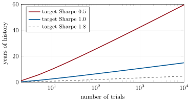
Minimum backtest length: the years of history below which the expected best of N independent null strategies reaches the target Sharpe ratio. Data: firm.overfit.min_backtest_length. — **Figure 20.3.** Minimum backtest length: the years of history below which the expected best of $N$ independent null strategies reaches the target Sharpe ratio. Data: `firm.overfit.min_backtest_length`.

20.4 Purged and embargoed cross-validation

Definition 20.5 (Label overlap, purging, embargo, combinatorial purged cross-validation)

Label overlap occurs when the targets of different observations share periods, as $h$ -day forward returns observed every day do. Purging removes from the training set every observation whose label overlaps in time the labels of the test set; an embargo also removes the training observations that immediately follow the test set, since features are serially correlated. Combinatorial purged cross-validation (CPCV) uses every choice of $k$ test folds out of $n$ , purged and embargoed, recombining the test folds into $\binom{n}{k}k/n$ backtest paths (López de Prado, 2018; as implemented in open-source libraries such as skfolio).

Shuffled $k$ -fold cross-validation, the default of general machine-learning libraries, puts neighbouring days into training and test sets alike. When labels overlap, a model can predict a test day’s label from the training days whose labels share its periods. The chapter’s demonstration is extreme on purpose: 20-day forward returns of pure noise, predicted by the five nearest neighbours in a feature that moves as slowly as time (a regime variable), five folds:

cross-validation	shuffled	contiguous	purged	purged and embargoed
$R^2$ of a forecast of noise	0.90	$-0.63$	$-0.57$	$-0.93$

Shuffled folds report that the model explains 90% of the variance of noise; every scheme that respects time says it is worse than a constant. Contiguous folds leak only at their edges, purging closes the edges, and the embargo guards against features that carry information across them. With a combinatorial scheme the same model can be judged on many paths instead of one, which turns a single out-of-sample Sharpe ratio into a distribution.

20.5 Walk-forward analysis

Definition 20.6 (Walk-forward analysis)

Walk-forward analysis repeats, through time, the cycle of choosing a strategy on a trailing window and trading it on the next period, and judges the stitched out-of-sample periods.

Walk-forward is the procedure the firm would actually follow, and it measures the procedure rather than a strategy. Re-choosing the best of the thousand systems every year on the previous five years gives a stitched Sharpe ratio of $-0.04$ on noise and 0.29 with the planted trend: the trend’s true Sharpe ratio, about what the average system earns, and twice what the in-sample winner of the whole search earned. Its limit is the single path: one history, one sequence of choices; CPCV and CSCV exist because one path is a small sample.

20.6 Practical defences

The defences are organisational before they are statistical. Count every trial, in the research log (chapter 1), including those abandoned; report the PBO of the search and the deflated Sharpe ratio of its winner (Book 4, chapter 12); fix the evaluation protocol before seeing the results; keep a holdout that nobody touches until the decision; prefer the broad region of parameters that works to its best point (a plateau, not a peak: here, the average system beat the winner); and demand a mechanism, because a mechanism survives the change of sample that a fitted number does not. Arnott, Harvey and Markowitz (2019) set these out as a protocol for research with machine learning; the PBO and the minimum backtest length put numbers on them.

20.7 Tutorial: one thousand trend systems

Goal. Search a thousand trend systems on noise and on a planted trend, estimate the PBO by CSCV, walk forward, compute the minimum backtest length, and compare four cross-validation schemes on overlapping labels. End state: Figures 20.1, 20.2 and 20.3; the table.

CSCV: block sums, then every split’s Sharpe ratios as matrix products, then the winner’s out-of-sample rank.

def cscv(M, n_blocks: int = 16, max_splits: int | None = None, seed: int = 0) -> dict:
    """M: (T, N) per-period returns of N strategies. Block sums and sums of squares make every split's in-sample and
    out-of-sample Sharpe ratios matrix products."""
    M = np.asarray(M, float)
    T, N = M.shape
    edges = np.linspace(0, T, n_blocks + 1).astype(int)
    s1 = np.array([M[a:b].sum(axis=0) for a, b in zip(edges[:-1], edges[1:], strict=True)])
    s2 = np.array([(M[a:b] ** 2).sum(axis=0) for a, b in zip(edges[:-1], edges[1:], strict=True)])
    n = np.diff(edges).astype(float)
    combos = [c for c in itertools.combinations(range(n_blocks), n_blocks // 2)]
    if max_splits is not None and len(combos) > max_splits:
        pick = np.random.default_rng(seed).choice(len(combos), max_splits, replace=False)
        combos = [combos[i] for i in sorted(pick)]
    A = np.zeros((len(combos), n_blocks))
    for i, c in enumerate(combos):
        A[i, list(c)] = 1.0

    def sharpe(W):
        cnt = W @ n
        mu = (W @ s1) / cnt[:, None]
        var = (W @ s2) / cnt[:, None] - mu ** 2
        return mu / np.sqrt(np.maximum(var, 1e-300))
    sr_is, sr_oos = sharpe(A), sharpe(1.0 - A)
    best = np.argmax(sr_is, axis=1)
    rows = np.arange(len(combos))
    oos_best = sr_oos[rows, best]
    rank = (sr_oos < oos_best[:, None]).sum(axis=1) + 1                    # 1 = worst ... N = best
    w = rank / (N + 1.0)
    logits = np.log(w / (1.0 - w))
    slope = np.polyfit(sr_is[rows, best], oos_best, 1)[0] if len(combos) > 2 else float("nan")
    return {"pbo": float(np.mean(logits <= 0.0)), "logits": logits, "is_best": sr_is[rows, best],
            "oos_of_best": oos_best, "slope": float(slope)}

Listing 20.1. The probability of backtest overfitting by CSCV. code/firm/overfit/firm_overfit.py

Purged k-fold with an embargo.

def purged_kfold(start, end, k: int = 5, embargo: int = 0) -> list[tuple[np.ndarray, np.ndarray]]:
    """start, end: (n,) index of the first and last period each observation's label uses, observations in time
    order. Test folds are contiguous; a training observation is dropped if its label interval overlaps the test
    fold's span (purging) or it starts within `embargo` periods after the fold's last label (embargo)."""
    start, end = np.asarray(start), np.asarray(end)
    n = len(start)
    out = []
    for f in np.array_split(np.arange(n), k):
        lo, hi = start[f].min(), end[f].max()
        overlap = (end >= lo) & (start <= hi)
        embargoed = (start > hi) & (start <= hi + embargo)
        train = np.flatnonzero(~overlap & ~embargoed)
        out.append((train, f))
    return out

Listing 20.2. Purging and embargo. code/firm/overfit/firm_overfit.py

Run search() for both worlds, walk_forward_sr(), minbtl(), label_leak() and fig_overfit.py.

What to change next. Choose the centre of the best plateau of parameters instead of the single best point and compare its out-of-sample Sharpe ratio; run CSCV on a hundred independent strategies instead of a thousand correlated ones and see the PBO approach one half on noise.

20.8 Build: the overfitting toolkit

Purpose. Every search the firm runs is reported with its probability of overfitting, its minimum backtest length, and cross-validation that respects time.

Interface. cscv(M, n_blocks, max_splits, seed), purged_kfold(start, end, k, embargo), cpcv(start, end, n_folds, n_test, embargo), cpcv_paths, walk_forward(n, train, test, step, anchored), min_backtest_length(n_trials, sr_target).

Rules. No shuffled cross-validation on time series; labels carry their start and end; the trial count comes from the research log, not memory.

Acceptance tests. code/firm/overfit/tests/: a PBO near one half and a non-positive slope on noise, near zero with one skilled strategy; purging and embargo by hand; CPCV’s fifteen splits and five paths, disjoint train and test sets; walk-forward windows, anchored and rolling; the minimum backtest length’s monotonicity and its quadrupling for half the target.

Stretch. CPCV Sharpe-ratio distributions for a model; the deflated Sharpe ratio from the effective number of trials; a PBO dashboard fed by the research log.

Sources and further reading

D. H. Bailey, J. M. Borwein, M. López de Prado and Q. J. Zhu, “The probability of backtest overfitting”, Journal of Computational Finance, 2016.
C. R. Harvey and Y. Liu, “Backtesting”, Journal of Portfolio Management 42(1), 2015.
M. López de Prado, Advances in Financial Machine Learning, Wiley, 2018; skfolio, CombinatorialPurgedCV (documentation of purging and embargo).
R. Arnott, C. R. Harvey and H. Markowitz, “A backtesting protocol in the era of machine learning”, Journal of Financial Data Science 1(1), 2019.

20.9 Exercises

Exercise 20.1 ★

In a CSCV split the in-sample winner ranks 380th of 1 000 out of sample (1 the worst). What is its logit, and does the split count toward the PBO?

Solution

Solution of Exercise 20.1.

$\omega = 380/1\,001 = 0.380$ , $\lambda = \ln(0.380/0.620) = -0.49$ : below the median, so the split counts toward the PBO.

Exercise 20.2 ★

How many backtest paths does CPCV give with 10 folds and 2 test folds? With 6 and 3?

Solution

Solution of Exercise 20.2.

$\binom{10}{2}\times 2/10 = 45 \times 2/10 = 9$ paths; $\binom{6}{3} \times 3/6 = 10$ .

Exercise 20.3 ★

Using the proposition’s approximation, how many years does a search over 100 trials need for a target Sharpe ratio of 1?

Solution

Solution of Exercise 20.3.

$2\ln 100/1^2 = 9.2$ years.

Exercise 20.4 ★★

Labels are 10-day forward returns observed daily; the test fold covers days 200 to 299. Which training days does purging remove, and which does an embargo of 5 days add?

Solution

Solution of Exercise 20.4.

A label observed on day $d$ spans days $d$ to $d + 9$ . The test labels span days 200 to 308. Purging removes the training days whose labels touch that span: 191 to 199 (their labels reach into day 200 and after) and 300 to 308 (they start inside it). An embargo of 5 days also removes days 309 to 313.

Exercise 20.5 ★★

Why can the PBO exceed one half? Explain with the thousand correlated trend systems.

Solution

Solution of Exercise 20.5.

Correlated systems share most of their noise; the in-sample winner is the one whose idiosyncratic part fitted the in-sample half best. With the halves drawn symmetrically, the same idiosyncratic part tends to fit the other half worse than the common part does for the others, so the winner falls below the median more often than not: selection anticorrelates with out-of-sample rank (the slopes of $-0.89$ and $-0.91$ ). With independent strategies and no skill the PBO is near one half.

Exercise 20.6 ★★

Why did the planted trend not make the in-sample winner a good choice, although every system earned the trend?

Solution

Solution of Exercise 20.6.

The trend is common to all systems: it lifts them all, by about the same amount, and does not distinguish among them. What distinguishes them in sample is noise, which does not persist; the winner of a search over noise on top of a common trend earns the trend minus its selection penalty (0.14 against an average of 0.26).

Exercise 20.7 ★★★

Coding. Run CSCV on the first 100 of the thousand systems only, and then on 100 independent noise strategies. Compare the PBOs and explain.

Solution

Solution of Exercise 20.7.

rs_overfit.pbo_hundred: 0.69 for the first 100 trend systems, 0.52 for 100 independent noise strategies. Independent strategies with no skill give a PBO near one half, as selection among pure noise should; correlated strategies push it above, because the winner’s edge is the part of its noise the others do not share.

Exercise 20.8 ★★★

Find the flaw. “We tuned the model’s hyperparameters by 10-fold cross-validation with shuffling, which is the standard, so the out-of-sample estimate is unbiased.”

Solution

Solution of Exercise 20.8.

Shuffled folds put overlapping labels and serially correlated features on both sides of every split: the model is scored on days whose labels it has, in effect, already seen. On the chapter’s noise, shuffled folds gave an $R^2$ of 0.90 and every time-respecting scheme a negative one. Use contiguous folds, purge overlapping labels, embargo after the test folds, and tune on folds that precede the test period.

20.10 Problem: One Thousand Trend Systems

Problem 20.1

Weekend problem — a search, measured

The chapter’s thousand trend systems on 25 years of synthetic returns, on noise and with a planted trend.

Part I — The search.

What are the best in-sample Sharpe ratio and its out-of-sample value on noise? With the trend?
What are the median in-sample and the average out-of-sample Sharpe ratios in each world?
What maximum would a thousand independent null strategies give over 17.9 years, and why is the observed winner lower?
What does the trend do to every system, and what does the search add?

Part II — The PBO.

How does CSCV compute a split’s Sharpe ratios quickly?
What are the PBOs and the degradation slopes in each world?
What does a PBO above one half mean?
What would the PBO be for one strategy with a real edge among noise?

Part III — Length and leakage.

Give the minimum backtest lengths for a thousand trials at targets of 0.5, 1 and 1.8.
Why does halving the target quadruple the length?
What $R^2$ do the four cross-validation schemes give for the forecast of noise?
Why do shuffled folds leak, and what do purging and embargo each remove?

Part IV — The verdict.

What Sharpe ratio does annual walk-forward re-selection give in each world?
State the named result: the PBO of the search and the deflated out-of-sample expectation of the chosen system.
Which would you trade: the in-sample winner, the average system, or the walk-forward procedure?
What should the research log contain for this search?
How would a mechanism change your confidence?
What does Harvey and Liu’s haircut add to the PBO?
Where does CPCV improve on walk-forward?
In one sentence: what is overfitting in a backtest search?

Solution

Solution of Problem 20.1.

Noise: 0.44 in sample, $-0.32$ out of sample. Trend: 0.77 and 0.14.
Noise: median in sample 0.17, average out of sample 0.20. Trend: 0.50 and 0.26.
0.77; the systems are highly correlated (their Sharpe ratios spread by 0.076), so the search amounts to few independent trials, and the expected best given that spread is 0.25 above the common level.
The trend lifts every system (median 0.50). The search adds a ranking that carries some information across the systems (correlation 0.33, the fifty best earn 0.29) but picks its single winner mostly for noise.
From block sums and sums of squares: each split is a set of blocks, so its means and variances are matrix products.
Noise: PBO 0.82, slope $-0.89$ . Trend: 0.74, slope $-0.91$ .
Selection is worse than choosing at random: the in-sample winner is more often than not below the median out of sample.
Near zero: it wins in sample and stays on top out of sample in almost every split (the build’s test finds below 1%).
42.4, 10.6 and 3.3 years.
The standard error of a Sharpe ratio falls with the square root of the history; to halve the target the error must halve, which takes four times the history.
Shuffled 0.90, contiguous $-0.63$ , purged $-0.57$ , purged and embargoed $-0.93$ .
Neighbouring days, whose labels share periods, fall into both sets; purging removes the training days whose labels overlap the test labels, the embargo the days just after the test set, whose features still carry its information.
$-0.04$ on noise, 0.29 with the trend.
Named result. The search’s PBO is 0.82 on noise and 0.74 with a real trend; the chosen system’s out-of-sample Sharpe ratio is $-0.32$ and 0.14, below the average system’s 0.20 and 0.26 in each world, while annual walk-forward re-selection earns $-0.04$ and 0.29. The deflated expectation of the winner is the average system’s, not its own in-sample 0.44 or 0.77.
The walk-forward procedure (or the average of the plateau), which earned the trend without paying for the choice of a point.
The thousand parameter pairs as trials, the data span, the selection rule, the PBO, the minimum backtest length and the deflated Sharpe ratio, before any out-of-sample look.
A reason for the trend (hedging pressure, slow diffusion) predicts that the broad class of systems should work, not a particular window, and points at the plateau rather than the peak.
A haircut of the reported Sharpe ratio for the number of tests, a single number to set beside the PBO’s probability.
Many out-of-sample paths instead of one, so the procedure’s performance is a distribution.
Choosing, among many backtests on limited history, the one whose success is the sample’s rather than the strategy’s.

20.11 Interview questions

Interview question 20.1 ★ researcher

You tested 500 strategies and the best has a Sharpe ratio of 2 in the backtest. What do you do next?

Solution

Solution of Interview question 20.1.

Record the 500 trials; compute the deflated Sharpe ratio of the best (Book 4, chapter 12) and the PBO of the search by CSCV; check the minimum backtest length for 500 trials at a Sharpe ratio of 2; look at the neighbourhood of the best (plateau or spike); find a mechanism; then test on data untouched by the search, or trade small (chapter 21).

Interview question 20.2 ★★ researcher, mle

Why is standard k-fold cross-validation wrong for financial time series, and what do you use instead?

Solution

Solution of Interview question 20.2.

Observations are serially correlated and labels overlap, so shuffled folds leak test information into training. Use contiguous folds with purging of overlapping labels and an embargo after each test fold, walk-forward for the procedure, and combinatorial purged cross-validation for a distribution of paths.

Interview question 20.3 ★★ researcher

Explain the probability of backtest overfitting and how CSCV estimates it.

Solution

Solution of Interview question 20.3.

The PBO is the probability that the in-sample winner of a search performs below the median out of sample. CSCV cuts the history into blocks, takes every symmetric split into in-sample and out-of-sample halves, picks the winner in sample and ranks it out of sample; the share of splits with a rank below the median estimates the PBO.

Interview question 20.4 ★★ researcher

How long must a backtest be to trust a Sharpe ratio of 1 found among 1 000 trials?

Solution

Solution of Interview question 20.4.

About $2\ln 1\,000 = 13.8$ years by the approximation, 10.6 with the exact expected maximum of independent trials; correlated trials need less, and a trustworthy answer needs more (to make the chance level well below the target, not equal to it).

Interview question 20.5 ★★ researcher, risk

What organisational practices reduce overfitting in a research team?

Solution

Solution of Interview question 20.5.

A research log with every trial counted; protocols fixed before results; a holdout guarded by someone else; review of searches by their PBO and deflated statistics; rewarding mechanisms and negative results; limits on the number of variants a project may try per year of data.

Interview question 20.6 ★★★ researcher

Derive the scaling of the minimum backtest length with the number of trials and the target Sharpe ratio.

Solution

Solution of Interview question 20.6.

Null Sharpe ratio estimates over $y$ years are about normal with variance $1/y$ ; the expected maximum of $N$ of them is about $\sqrt{2\ln N}/\sqrt y$ ; setting it equal to the target $s$ gives $y = 2\ln N/s^2$ : logarithmic in the number of trials, inverse square in the target.

Terms defined in this chapter

See all 2333 terms in the glossary