Research Craft: Predictors, Backtests, Measurement, Portfolios · Research

27Transaction Costs in Research

A daily forecast of fifty large stocks has a gross Sharpe ratio of 2.56. Traded as the mean–variance book it implies, by a fund of $1 billion, it turns over 5.33 times its capital a day and pays 1 223 per cent of its capital a year in costs: a Sharpe ratio of $-29$ after costs. The same forecast with the costs inside the optimiser nets 1.80; smoothed over a day as well, 2.43. Nothing about the signal changed. Costs are not a haircut applied to a finished backtest; they belong in the model of the market, in the optimiser and in the signal, and they depend on the fund’s size. This chapter fits a cost model to the firm’s fills, puts it inside the construction with firm.tcost, nets strategies’ trades against each other, and makes signals cost-aware.

27.1 Cost models

Definition 27.1 (Temporary impact, permanent impact, square-root impact law, percentage of volume)

The temporary impact of a trade is the part of its price concession that decays after the trade; the permanent impact is the part that remains, the information the market reads in it. An order’s percentage of volume is its size $Q$ over the market’s daily volume $V$ . The square-root impact law states that an order’s average impact, as a fraction of price, is about $\eta\,\sigma\sqrt{Q/V}$ for daily volatility $\sigma$ and a constant $\eta$ of order one.

A trade’s cost has three parts: half the bid–ask spread (Book 1, chapter 1), fees, and market impact (chapter 18). The first two are linear in the size traded; impact is not. Tóth and co-authors explained the square root by a supply and demand that vanish at the current price, so that a large order must be cut up and digested; Almgren, Thum, Hauptmann and Li, fitting almost 700 000 orders executed by Citigroup’s US equity desks, found the temporary impact grew as the 3/5 power of the trading rate. The exponent near a half matters more than its precise value: a trade twice as large costs more per share, and so the cost of a book is not proportional to its size.

27.2 Estimating costs from your own fills

The firm’s cost model comes from its own parent orders. The chapter simulates a year of them, 5 000 orders with sizes from 0.01% to 20% of daily volume and daily volatilities from 1% to 3%, from a planted law: half a spread of 2 basis points and impact $0.7\,\sigma\sqrt{Q/V}$ , plus the price’s own move while the order works. The move is the difficulty. At 1% of daily volume and 2% volatility the planted impact is 14 basis points; the price’s move over the order’s life has a standard deviation of 63. A single order says almost nothing about its cost, and a cost model is a regression on thousands of orders, whose noise grows with the order’s size.

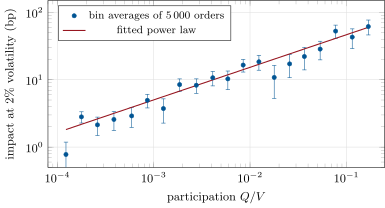
firm.tcost.fit_impact (Listing 27.1) averages the costs within twenty bins of participation, fits the exponent on the logarithms of the bin averages, and fits $\eta$ with the exponent held at a half, with a standard error robust to the growing noise. From 5 000 orders it recovers $\eta = 0.71$ (standard error 0.08) and an exponent of 0.48 (0.03); from 500 orders, $1.09$ (0.24) and 0.59 (0.07); from 50 000, $0.67$ (0.03) and 0.49 (0.01) (Figure 27.1). A desk with a few hundred orders a year knows its cost coefficient to within a third; Kyle and Obizhaeva’s invariance hypotheses, supported on more than 400 000 portfolio-transition orders, are one way to borrow strength across stocks by scaling costs with each stock’s volume and volatility.

Impact estimated from a simulated year of parent orders (half spread removed, scaled to 2% daily volatility), with two-standard-error bars and the fitted law. The smallest orders’ bins are the noisiest relative to their cost. Data: rs_tcost.fills. — **Figure 27.1.** Impact estimated from a simulated year of parent orders (half spread removed, scaled to 2% daily volatility), with two-standard-error bars and the fitted law. The smallest orders’ bins are the noisiest relative to their cost. Data: `rs_tcost.fills`.

27.3 Costs inside the optimiser

Definition 27.2 (Cost-aware optimisation)

Cost-aware optimisation maximises $\alpha^\top w - \frac\gamma2 w^\top\Sigma w - C(w - w_0)$ , with $C$ the cost model of the trade from the current book: here $C(d) = \sum_i s_i\lvert d_i\rvert + \eta\sigma_i\lvert d_i\rvert^{3/2}\sqrt{A/V_i}$ for half spreads $s_i$ , a fund of size $A$ and daily traded values $V_i$ .

The $3/2$ power makes the problem a second-order cone programme (Book 4, chapter 23). firm.tcost.cost_aware solves it by accelerated proximal gradient instead: the quadratic part is smooth, the cost is separable, and its proximal step has a closed form, a soft threshold by the spread followed by the root of a quadratic in $\sqrt{\lvert d\rvert}$ (Listing 27.2). The chapter’s books hold chapter 26’s fifty names long and short, daily; the forecast is the true expected return of the three planted signals plus noise one and a half times as large, new every day, and $\gamma = 72$ . The daily traded values of these names have a median of $474 million.

fund size	$10 million	$100 million	$1 billion	$10 billion
mean–variance, costs ignored: after costs	$-4.96$	$-15.91$	$-29.47$	$-34.0$
costs inside: Sharpe ratio before costs	3.12	3.14	3.06	2.11
after costs	$-0.31$	0.06	1.80	1.76
costs a year	46.1%	28.8%	7.6%	1.2%
daily turnover	2.269	0.814	0.148	0.018
costs inside, forecast smoothed over one day	1.68	2.03	2.43	1.66
costs ignored, forecast smoothed over fifty days	1.78	1.63	1.15	$-0.23$

The book that ignores costs trades 5.33 times its capital a day; even a $10 million fund, which pays little more than the spread, loses. The cost-aware book has a surprise at the small end: it loses at $10 million and wins at $1 billion. With cheap trading it believes its forecast and chases its daily noise, which the optimiser cannot tell from alpha; at $1 billion the cost of trading forces it to move slowly, and moving slowly averages the noise away, so that its Sharpe ratio before costs (3.06) is higher than the naive book’s (2.56). Costs in the optimiser protect a book from its forecast’s noise only when they are large relative to that noise; below that, the forecast itself must be made slower.

27.4 Netting across strategies

Definition 27.3 (Internal crossing)

Internal crossing nets the trades of a firm’s strategies in the same stock before any reach the market: a buy of one strategy and a sell of another cross at no market cost.

Two teams trading the same fifty names from their own forecasts of the same truth, each with its own noise, each smoothed over twenty days and each running $1 billion, would pay 8.27% and 8.73% of a team’s capital a year apart. Netted, their trades cost 16.04%: a saving of 0.96 points, 5.7% of the total. The saving is smaller than the offsetting trades suggest, because netting cuts both ways under a concave impact law. Where the teams trade opposite ways, the netted trade is smaller and cheaper; where they trade the same way, the combined trade is larger and, cost growing as the $3/2$ power, dearer than the two apart: 2.94 points a year dearer here. Each team’s own cost estimate understates what its trades cost the firm when others trade alongside it, the first appearance of crowding (chapter 28). firm.tcost.netting_saving shares the saving out in proportion to each strategy’s standalone cost, so that netting never makes a strategy’s reported costs worse.

27.5 Cost-aware signals

Definition 27.4 (Signal smoothing, break-even cost)

Signal smoothing replaces a forecast by an exponentially weighted average of its recent values, with a half-life chosen for net performance. A strategy’s break-even cost is the cost per unit traded at which its return after costs is zero: its gross return over its turnover.

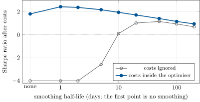
Smoothing trades signal for turnover. It delays the forecast, which loses the part of the alpha that decays fast, and it averages the forecast’s noise, which removes trading that had no reason. Figure 27.2 shows the net Sharpe ratio against the half-life at $1 billion. The book that ignores costs rises from $-29.47$ to a peak of 1.15 at fifty days, and falls beyond it (0.93 at a hundred days, 0.69 at two hundred) as the delay costs more signal than it saves in costs. The cost-aware book peaks early, at 2.43 with a one-day half-life, because the optimiser already smooths; long half-lives only cost it signal (0.94 at two hundred days). The optimal smoothing depends on who does the rest of the smoothing, and chapter 26’s aim portfolio is the same idea made exact for signals whose decay rates are known.

The net Sharpe ratio of the fifty-name book at $1 billion against the half-life of the forecast’s smoothing; values below -4 are drawn at -4. Data: rs_tcost.smoothing_curve. — **Figure 27.2.** The net Sharpe ratio of the fifty-name book at $1 billion against the half-life of the forecast’s smoothing; values below $-4$ are drawn at $-4$ . Data: `rs_tcost.smoothing_curve`.

27.6 Tutorial: from 2.56 to $-29$ and back

Goal. Fit the impact law to simulated fills, trade the fifty-name forecast with costs ignored and inside the optimiser at four fund sizes, smooth the forecast, and net two teams’ trades. End state: the table, Figures 27.1 and 27.2.

The fit: binned averages for the exponent, the robust fit for $\eta$ .

def fit_impact(cost, sigma, participation, half_spread, bins: int = 20):
    """cost: realised cost of each parent order as a fraction of value (signed so that positive is a loss), sigma:
    daily volatility, participation: Q / V. Averages within participation bins remove most of the price noise; the
    exponent comes from log(mean cost - half spread) on log participation, eta from the fit with exponent 1/2."""
    c, s, p = (np.asarray(a, float) for a in (cost, sigma, participation))
    y = (c - half_spread) / s
    edges = np.quantile(p, np.linspace(0, 1, bins + 1))
    idx = np.clip(np.searchsorted(edges, p, side="right") - 1, 0, bins - 1)
    xm = np.array([p[idx == k].mean() for k in range(bins)])
    ym = np.array([y[idx == k].mean() for k in range(bins)])
    se_m = np.array([y[idx == k].std(ddof=1) / math.sqrt((idx == k).sum()) for k in range(bins)])
    ok = ym > 0
    X = np.column_stack([np.ones(ok.sum()), np.log(xm[ok])])
    wts = (ym[ok] / se_m[ok]) ** 2                                       # delta method: var(log m) = (se / m)^2
    A = X.T @ (wts[:, None] * X)
    beta = np.linalg.solve(A, X.T @ (wts * np.log(ym[ok])))
    cov = np.linalg.inv(A)
    root = np.sqrt(p)
    eta = float(root @ y / (root @ root))
    resid = y - eta * root
    se_eta = float(math.sqrt((root**2 * resid**2).sum()) / (root @ root))      # robust: the noise grows with size
    return {"eta": float(math.exp(beta[0])), "exponent": float(beta[1]), "se_exponent": float(math.sqrt(cov[1, 1])),
            "eta_fixed": eta, "se_eta": se_eta}

Listing 27.1. Estimating the impact law from fills. code/firm/tcost/firm_tcost.py

The cost-aware book: the closed-form proximal step and the accelerated iteration.

def prox_cost(v, s, c):
    """Minimise (x - v)^2 / 2 + s|x| + c|x|^(3/2): shrink |v| by s, then y = sqrt(x) solves y^2 + 1.5 c y = |v| - s."""
    v, s, c = (np.asarray(a, float) for a in (v, s, c))
    r = np.maximum(np.abs(v) - s, 0.0)
    y = (-1.5 * c + np.sqrt((1.5 * c) ** 2 + 4 * r)) / 2
    return np.sign(v) * y * y


def cost_aware(alpha, Sigma, w0, aum: float, sigma, adv, half_spread, eta: float, gamma: float,
               neutral: float = 0.0, iters: int = 500, tol: float = 1e-12):
    """FISTA on f(w) = gamma/2 w'Sigma w - alpha'w + neutral/2 (1'w)^2 with the separable cost as the proximal term
    (in d = w - w0: s_i |d_i| + c_i |d_i|^(3/2), c_i = eta sigma_i sqrt(aum / adv_i))."""
    alpha, Sigma, w0 = (np.asarray(a, float) for a in (alpha, Sigma, w0))
    n = len(alpha)
    Hm = gamma * Sigma + neutral * np.ones((n, n))
    L = float(np.linalg.eigvalsh(Hm).max())
    s = np.asarray(half_spread, float) * np.ones(n)
    c = eta * np.asarray(sigma, float) * np.sqrt(aum / np.asarray(adv, float))
    w = w0.copy()
    z, tk = w.copy(), 1.0
    for _ in range(iters):
        g = Hm @ z - alpha
        new = w0 + prox_cost(z - g / L - w0, s / L, c / L)
        t1 = (1 + math.sqrt(1 + 4 * tk * tk)) / 2
        z = new + (tk - 1) / t1 * (new - w)
        if np.abs(new - w).max() < tol:
            w = new
            break
        w, tk = new, t1
    return w

Listing 27.2. Mean–variance with spread and power-law impact inside. code/firm/tcost/firm_tcost.py

Run rs_tcost.estimate(n), run(book, aum, half_life), smoothing_curve, netting and fig_tcost.py.

What to change next. Make the forecast’s noise persistent (an autoregression rather than new each day) and watch the optimal smoothing lengthen; add linear costs only and see the cost-aware book’s no-trade region appear.

27.7 Build: the cost toolkit

Purpose. One cost model, estimated from the firm’s fills and used everywhere: in backtests, in the optimiser, in capacity estimates and in the netting of strategies.

Interface. impact_bp(eta, sigma, participation, exponent), fit_impact(cost, sigma, participation, half_spread), trade_cost(dw, aum, sigma, adv, half_spread, eta, fee), prox_cost(v, s, c), cost_aware(alpha, Sigma, w0, aum, sigma, adv, half_spread, eta, gamma, neutral), net_trades, netting_saving(lists, cost_fn), smooth(signal, half_life), breakeven_cost.

Rules. Costs depend on fund size and are always charged at the size the strategy will run; the cost model is re-fitted on the firm’s fills with standard errors; no strategy is judged before costs; netting savings are shared so that no strategy’s costs rise because of another.

Acceptance tests. code/firm/tcost/tests/: the planted law recovered within its standard errors; the proximal step optimal on a fine grid; the cost of a trade by hand; the cost-aware book equal to mean–variance without costs, and locally optimal with them; netting by hand; the smoothing’s step response; break-even.

Stretch. Temporary and permanent impact with decay (a propagator); costs per venue and time of day; multi-period cost-aware construction.

Sources and further reading

B. Tóth et al., “Anomalous price impact and the critical nature of liquidity in financial markets”, Physical Review X 1, 021006, 2011.
R. Almgren, C. Thum, E. Hauptmann and H. Li, “Direct estimation of equity market impact”, Risk, 2005.
A. S. Kyle and A. A. Obizhaeva, “Market microstructure invariance: empirical hypotheses”, Econometrica 84(4), 2016.
J.-P. Bouchaud, J. Bonart, J. Donier and M. Gould, Trades, Quotes and Prices, Cambridge University Press, 2018.

27.8 Exercises

Exercise 27.1 ★

What does an order of 5% of daily volume cost in a stock of 2% daily volatility, with a half spread of 2 basis points and $\eta = 0.7$ ?

Solution

Solution of Exercise 27.1.

$2 + 10\,000 \times 0.7 \times 0.02 \times \sqrt{0.05} = 2 + 31.3 = 33.3$ basis points.

Exercise 27.2 ★

The naive book earns 49.1% a year before costs and trades 5.33 times its capital a day. What is its break-even cost per unit traded?

Solution

Solution of Exercise 27.2.

$0.491/(5.33 \times 252) = 3.66$ basis points per unit traded; its half spread alone is 2, and impact at $1 billion is far above the rest.

Exercise 27.3 ★

Two strategies each trade $q$ in the same direction under a cost growing as $q^{3/2}$ . By how much does the netted trade cost more than the two apart?

Solution

Solution of Exercise 27.3.

Apart: $2q^{3/2}$ ; netted: $(2q)^{3/2} = 2^{3/2}q^{3/2}$ ; the netted trade costs $(2^{3/2} - 2)/2 = 41\%$ more.

Exercise 27.4 ★★

Why does a single parent order say almost nothing about the firm’s cost coefficient? How many would you want?

Solution

Solution of Exercise 27.4.

Its cost is dominated by the price’s move while it works (63 basis points of standard deviation at 1% participation against 14 of impact). The coefficient is an average over orders: 500 orders pin $\eta$ to within about a third (0.24 around 1.09), 5 000 to about 12% (0.08 around 0.71), 50 000 to 4%.

Exercise 27.5 ★★

Why does the cost-aware book lose at $10 million but win at $1 billion?

Solution

Solution of Exercise 27.5.

The optimiser trades whenever the forecast’s change pays for the cost. At $10 million costs are small, so it follows the forecast’s daily noise, which is not alpha, and pays 46.1% a year to do so. At $1 billion costs make it move slowly, which averages the noise; it even earns more before costs.

Exercise 27.6 ★★

Derive the proximal step of $s\lvert x\rvert + c\lvert x\rvert^{3/2}$ .

Solution

Solution of Exercise 27.6.

For $v > 0$ the minimiser of $\frac12(x - v)^2 + s\lvert x\rvert + c\lvert x\rvert^{3/2}$ is non-negative; if $v \le s$ it is 0; otherwise the first-order condition $x - v + s + \frac32 c\sqrt x = 0$ gives, with $y = \sqrt x$ , $y^2 + \frac32 cy - (v - s) = 0$ , so $y = \frac12(-\frac32 c + \sqrt{\frac94 c^2 + 4(v - s)})$ and $x = y^2$ ; by symmetry the sign of $v$ is restored.

Exercise 27.7 ★★★

Coding. Run rs_tcost.smoothing_curve for both books and explain why their optimal half-lives differ.

Solution

Solution of Exercise 27.7.

Costs ignored: $-29.47$ raw, rising to 1.15 at fifty days and falling to 0.69 at two hundred. Costs inside: 1.80 raw, 2.43 at one day, 0.94 at two hundred. The cost-aware optimiser already smooths the book through its reluctance to trade, so it needs only a little smoothing of the forecast; the naive book gets all its smoothing from the forecast.

Exercise 27.8 ★★★

Find the flaw. “Impact follows a square root, so our costs grow with the square root of our assets: doubling the fund costs only 41% more.”

Solution

Solution of Exercise 27.8.

The cost per unit traded grows as the square root of the size of each trade, so as a fraction of capital the costs rise by $\sqrt 2 = 1.41$ times when the fund doubles; in dollars they rise $2^{3/2} = 2.83$ times, while the gross dollars only double. The fund’s return after costs falls with size, and past some size its dollar profit falls too (chapter 28).

27.9 Problem: From 2.56 to $-29$

Problem 27.1

Weekend problem — a signal, costed

The chapter’s simulated fills and fifty-name books.

Part I — The cost model.

State the planted cost law and the size of the price noise at 1% participation.
What do 500, 5 000 and 50 000 orders recover for $\eta$ and the exponent?
What did Almgren and co-authors and Tóth and co-authors find for the exponent?
Why is the fit done on bin averages, and why a robust standard error?

Part II — The books.

What do the naive book’s turnover, costs and net Sharpe ratio come to at $1 billion?
Give the cost-aware book’s net Sharpe ratios at the four fund sizes.
Why is its Sharpe ratio before costs higher than the naive book’s?
What happens at $10 billion?

Part III — Netting and smoothing.

What do the two teams’ costs come to apart and netted?
Why does netting cost more on same-direction trades?
What are the net Sharpe ratios against the half-life for both books?

Part IV — The verdict.

State the named result: the net Sharpe ratio against the smoothing half-life, and the optimal smoothing.
Which book would you run at $1 billion?
What fund size would you advise for the smoothed naive book?
How should a research report present a strategy’s costs?
Where would a propagator model of impact change the conclusions?
How would you estimate the firm’s cost model if it had no fills yet?
What does netting imply for the capacity of several strategies trading the same names?
How does chapter 26’s aim portfolio relate to smoothing?
In one sentence: where do costs belong in research?

Solution

Solution of Problem 27.1.

Half spread 2 basis points plus $0.7\sigma\sqrt{Q/V}$ ; at 1% participation and 2% volatility, 14 basis points of impact against a price noise of 63.
500: $\eta = 1.09$ (0.24), exponent 0.59 (0.07); 5 000: 0.71 (0.08), 0.48 (0.03); 50 000: 0.67 (0.03), 0.49 (0.01).
Almgren and co-authors: a 3/5 power on about 700 000 Citigroup orders; Tóth and co-authors: the square root.
Averages within bins remove most of the price noise before taking logarithms; the noise grows with the order’s size, so a homoskedastic standard error is wrong.
Turnover 5.33 a day, costs 1 223% a year, net Sharpe ratio $-29.47$ .
$-0.31$ , 0.06, 1.80 and 1.76.
It trades slowly and so averages the forecast’s daily noise.
Costs make it trade 0.018 of capital a day; its Sharpe ratio before costs falls to 2.11 as the book cannot follow even the slow signals, and nets 1.76.
8.27% and 8.73% of a team’s capital a year apart; 16.04% netted, a saving of 0.96 points (5.7%).
Cost grows as the $3/2$ power of the trade: the combined trade is dearer than the two apart (2.94 points a year here).
Costs ignored: $-29.47$ , $-19.18$ , $-10.62$ , $-2.57$ , 0.10, 1.02, 1.15, 0.93, 0.69 for no smoothing and half-lives of 1, 2, 5, 10, 20, 50, 100, 200 days. Costs inside: 1.80, 2.43, 2.37, 2.17, 1.94, 1.71, 1.40, 1.15, 0.94.
Named result. The net Sharpe ratio peaks at a half-life of fifty days (1.15) for the book that ignores costs and at one day (2.43) for the cost-aware book, at $1 billion.
The cost-aware book on the forecast smoothed over one day (2.43).
Small: its net ratio falls from 1.78 at $10 million to 1.15 at $1 billion and $-0.23$ at $10 billion.
With the cost model, the fund size assumed, the costs a year, turnover, break-even cost, and net results at several sizes.
When trades follow each other within the impact’s decay time, as the daily book’s do: a propagator charges the second trade for the first’s remaining impact.
From its brokers’ pre-trade models or published estimates, scaled by volume and volatility (invariance), and replace it with its own fits as fills come in.
Their capacities are not additive: trades in the same direction add up under a concave law, so the firm’s capacity is less than the sum.
Both slow the book towards the persistent part of the forecast; the aim portfolio does it with known decay rates, smoothing with a chosen half-life.
In the model of the market, in the optimiser and in the signal, at the size the strategy will run.

27.10 Interview questions

Interview question 27.1 ★ trader, researcher

How does market impact scale with order size? What evidence is there?

Solution

Solution of Interview question 27.1.

Concavely: average impact grows roughly as the square root of the order’s size relative to daily volume, scaled by volatility. Evidence: Almgren and co-authors on about 700 000 Citigroup orders (a 3/5 power for temporary impact), Tóth and co-authors (square root), and invariance studies of portfolio transitions.

Interview question 27.2 ★★ researcher

Your signal has a daily Sharpe ratio of 2.5 before costs. What do you do before you believe it?

Solution

Solution of Interview question 27.2.

Measure its turnover and break-even cost, cost it at the fund size it will run with a fitted impact model, build it with costs inside the optimiser, smooth it, and look at the decay of its information coefficient: a daily 2.5 before costs can be negative after them.

Interview question 27.3 ★★ trader

How would you estimate your desk’s market impact from its own fills?

Solution

Solution of Interview question 27.3.

Record each parent order’s decision and arrival prices, fills, size, participation, volatility and volume; regress cost (net of half spread) on $\sigma\sqrt{Q/V}$ with robust errors and fit the exponent on binned averages; control for the market’s move; use thousands of orders and re-fit regularly.

Interview question 27.4 ★★ researcher, developer

How do you put a $3/2$ -power cost into a portfolio optimiser?

Solution

Solution of Interview question 27.4.

As a second-order cone constraint ( $t_i \ge \lvert d_i\rvert^{3/2}$ is representable with rotated cones), or, as here, by a proximal method: the cost is separable and its proximal step has a closed form, a soft threshold followed by the root of a quadratic in $\sqrt{\lvert d\rvert}$ .

Interview question 27.5 ★★ researcher, trader

Two of the firm’s strategies trade the same stocks. What should the firm do about it?

Solution

Solution of Interview question 27.5.

Net their trades internally, share the saving by standalone cost, and cost each strategy at its marginal cost to the firm: same-direction trades cost more together than apart, so combined capacity is below the sum.

Interview question 27.6 ★★★ researcher

Show that with costs growing as the $3/2$ power of the trade, a strategy’s return after costs is maximised at a finite fund size, and find it for a constant gross return.

Solution

Solution of Interview question 27.6.

If the gross return is $g$ a year on capital $A$ and costs as a fraction of capital grow as $k\sqrt A$ (trades scale with $A$ , cost per unit with $\sqrt A$ ), the dollar profit is $gA - kA^{3/2}$ , maximised at $A^* = (2g/(3k))^2$ , where the return on capital is $g/3$ ; beyond it every dollar added lowers the profit.

Terms defined in this chapter

See all 2333 terms in the glossary

27.1 Cost models

27.2 Estimating costs from your own fills

27.3 Costs inside the optimiser

27.4 Netting across strategies

27.5 Cost-aware signals

27.6 Tutorial: from 2.56 to −29-29−29 and back

27.7 Build: the cost toolkit

27.8 Exercises

27.9 Problem: From 2.56 to −29-29−29

27.10 Interview questions

Terms defined in this chapter

27.6 Tutorial: from 2.56 to $-29$ and back

27.9 Problem: From 2.56 to $-29$