12Alternative and Text Data

A vendor offers five years of card-spending data on four hundred retailers for a fee of several hundred thousand dollars a year. The trial file arrives with a note: the panel changed card provider in its third year. The history looks excellent. The questions are the chapter’s: what exactly is this dataset, which of its history was known at the time, what does it add to what the firm already has, is it legal to use, and what is it worth. Froot, Kang, Ozik and Sadka built real-time proxies of retail sales from sources including about 50 million mobile devices and found that their within-quarter measure explained sales growth and earnings surprises, with average excess returns at announcement of 3.4%; Zhu (2019) found that the introduction of consumer-transaction and satellite data increased the informativeness of prices. Such data work. The purchase is a research project of its own, with a harness (firm.vendoreval), a synthetic trial whose truth is planted, and a decision at the end.

12.1 What the datasets are

Definition 12.1 (Alternative data, panel drift)

Alternative data are data about companies, economies or markets from sources other than prices, filings and official statistics: card and bank transactions, receipts, web traffic and prices, app usage, geolocation, satellite and aerial images, shipping and flight records, job postings, text. A dataset built on a panel (of cardholders, devices, stores) suffers panel drift when the panel’s composition or its relation to the quantity it measures changes over time: a provider change, attrition, a new source, a re-weighting.

Every alternative dataset is a measurement process with a history of its own, and three questions come before any backtest. What is measured, by whom, and with what consent (the provenance)? When was each historical value first delivered (the knowledge time of chapter 3)? How has the panel changed (its drift)? The last two are usually tangled: a vendor launches, then reconstructs years of history from today’s panel to sell a longer backtest, and the reconstruction is fitted, knowingly or not, to outcomes that were known when it was built. That is backfill bias (chapter 3) in its commercial form.

12.2 Evaluating a vendor

Definition 12.2 (Data trial, incremental information coefficient)

A data trial is a time-limited evaluation of a dataset under a trial licence, before purchase. The incremental information coefficient of a new feature is the information coefficient of its residual after regressing it, cross-section by cross-section, on the features the firm already owns.

The chapter’s trial is synthetic and its story planted, so every conclusion can be checked. In firm.synthmkt, 400 names listed for all ten years are the retailers; each quarter’s true earnings surprise is announced a random number of days after the quarter’s end, with a price jump in its direction. The vendor’s panel value for each retailer and quarter is delivered ten trading days after the quarter ends. Its five-year history (years 6 to 10 of the market) hides three things: the vendor went live when it changed provider, at the start of the history’s third year; the first two years were reconstructed at launch from the new provider’s panel, re-weighted to match the retailers’ reported results; and the live panel covers fewer names, with a level shift and more noise. The firm already owns a signal that carries part of the same information. The trial keeps only quarters whose announcement falls after the delivery, 5 980 rows, and firm.vendoreval measures what it can see.

Coverage and history. The backfilled years have 338 rows a quarter, the live years 273: the sample shrank when the product went live, the opposite of a growing panel, and a clue. Of all rows, 39.6% were first delivered more than a quarter after their period (the vendor’s own launch date, which the trial must ask for, dates them).

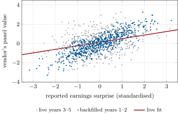
The relation to the truth. Regressing the panel value on the reported surprise year by year (Figure 12.1): slope 0.92 and 0.87 in the first two years, 0.37, 0.39 and 0.35 after; correlation 0.85 and 0.84, then 0.35, 0.35 and 0.32; an intercept of 0.02 before and 0.12 to 0.17 after. A CUSUM of the residuals, ordered in time (chapter 13), puts the single most likely break at the start of the third year, with a statistic of 3.05 (the 5% critical value is about 1.36). The provider change the vendor mentioned is also where the history stops being a reconstruction.

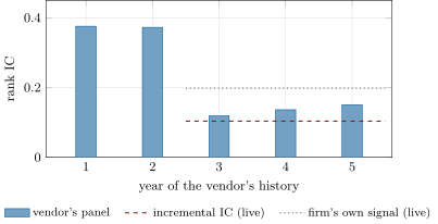
The information coefficient by year with the return from delivery to announcement: 0.38 and 0.37 in the backfilled years, 0.12, 0.14 and 0.15 in the live ones (Figure 12.2). A backtest over the whole history would report the average of the two regimes and describe neither.

What is new. In the live years the firm’s own signal has an IC of 0.20, larger than the vendor’s 0.13. Residualised on it quarter by quarter, the vendor’s feature keeps an incremental IC of 0.10, with a $t$ statistic of 4.0 over 12 quarters: the panel carries information the firm lacks, less than its raw IC suggests.

The real-data counterparts of each step are well known to anyone who has run trials: coverage tables with gaps where a merchant left the panel, histories whose first delivery date the vendor cannot supply, tickers mapped with today’s security master (chapter 4), data revised without notice. The harness asks the same questions of any file.

12.3 Text as data

Definition 12.3 (Dictionary method, sentiment score, document embedding)

A dictionary method scores a document by counting the words it contains from fixed word lists. A sentiment score is such a measure of tone, for instance the share of negative words, or negative minus positive words over all words. A document embedding maps a document to a vector of real numbers (word counts weighted by rarity, or the output of a trained language model) so that documents with similar content have nearby vectors.

Tetlock (2007) measured the pessimism of a daily Wall Street Journal column and found that high media pessimism predicts downward pressure on market prices followed by a reversion to fundamentals, and that unusually high or low pessimism predicts high trading volume. Loughran and McDonald (2011) showed that word lists built for other disciplines misclassify common words in financial text: in 10-Ks from 1994 to 2008, almost three-fourths of the words the widely used Harvard dictionary classifies as negative are not negative in financial contexts (liability, tax, cost, capital), and they built finance-specific lists.

The chapter’s corpus plants that problem. Two thousand synthetic documents of 400 words have a tone $\tau$ that raises the rate of eight positive words and lowers that of eight negative ones; eight finance words that a general list calls negative are frequent and unrelated to tone, and make 77% of the general list’s negative hits. The negative-word share correlates with $-\tau$ at 0.74 with the general list, 0.87 with the finance list, and 0.95 for negative minus positive words with the finance lists. The numbers are the corpus’s; the lesson is Loughran and McDonald’s: a dictionary is a measurement instrument, calibrated for a domain.

Embeddings replace hand-built lists with learned representations and move the problems rather than solving them. Their training corpus has a date, and a model trained on text written after the backtest’s decision date knows how the story ended; its vocabulary and its sense of what is similar drift with each version; and the mapping from embedding to return is one more fitted model, with the overfitting risks of chapter 20. The point-in-time rule applies to the model as to the data: the model used at a decision date is one that existed then.

12.4 Law and ethics

Definition 12.4 (Material non-public information)

Material non-public information (MNPI) is information about a security or its issuer that has not been made public and that is material: in the SEC’s words, a matter is material if there is a substantial likelihood that a reasonable person would consider it important. Trading on MNPI obtained in breach of a duty is insider trading.

Alternative data sit near that line by design: they are valuable because they are not in the filings. The legal questions are about how the data were obtained and whether the seller had the right to sell them, and a buyer’s diligence is part of its own defence.

As of September 2026 — Alternative data in enforcement and litigation

In September 2021 the SEC settled securities fraud charges against App Annie, an alternative data provider for the mobile app industry, and its co-founder, who agreed to pay more than $10 million: the SEC’s first enforcement action charging an alternative data provider with securities fraud. The order found that, while telling companies their confidential app data would be aggregated and anonymised, App Annie used non-aggregated, non-anonymised data from late 2014 to mid-2018 to alter its estimates and make them more valuable to trading firms, and misrepresented this to those firms. In April 2022 the US Court of Appeals for the Ninth Circuit, in hiQ Labs v. LinkedIn, again affirmed a preliminary injunction letting a data analytics company access publicly available LinkedIn profiles, holding that the Computer Fraud and Abuse Act’s concept of access “without authorization” does not apply to public websites. In the European Union, the General Data Protection Regulation (Regulation 2016/679) defines personal data as any information relating to an identified or identifiable natural person, identifiable directly or indirectly, including by location data or an online identifier.

A research team’s checklist follows from these cases: the vendor’s written representation of how the data were collected and with which consents; whether any source is an insider or bound by confidentiality; whether personal data are present, pseudonymised or truly aggregated; the terms of service of scraped sites (a preliminary injunction on public profiles under one statute is not a licence to scrape); a legal and compliance sign-off before the trial, not after the purchase; and a record of all of it, kept with the dataset’s metadata. The ethics are wider than the law: data that let a desk infer who visited a clinic are not acceptable because a court has not yet ruled on them.

12.5 The buy decision

The value of a dataset is the profit of what it adds, net of costs, over the life of the contract, as the edge decays because other buyers trade on it. In the trial, the long–short spread of the top and bottom quintiles of the incremental feature earns 2.9% a quarter in the live years (live raw feature: 3.4%; the backfilled years: 10.4%). With the desk’s capacity for announcement trades in these names put at $20 million, trading costs of 0.4% a year and a two-year half-life for the edge, the break-even annual fee over a three-year contract is $1.35 million. The vendor’s history, taken at face value, implies $5.06 million; the live raw feature $1.59 million (Figure 12.3). The half-life decides the rest: at six months the incremental break-even is $0.43 million, near the asking price.

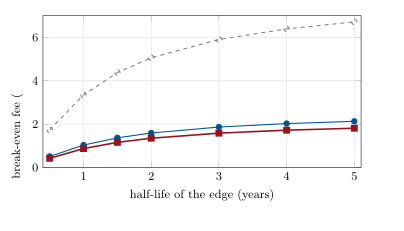
Three corrections separate the pitch from the price: live data only (the backfill tripled the spread), incremental over what is owned (a further 15%), and decay (a factor of three between a six-month and a two-year half-life). The half-life is the hardest to know before buying: it depends on how many others buy the same file, which the vendor knows and the buyer does not; chapter 28 measures it after the fact. Capacity (chapter 28) and costs (chapter 27) come from the firm’s own models. The chapter’s weekend problem makes the decision.

12.6 Predictor cards

Predictor card 12.1 — Card-panel sales surprise

Definition. The panel’s spending growth for the quarter, residualised on the firm’s existing signals, ranked across the retailers announcing in the next weeks.

Inputs and timestamps. The vendor’s quarterly values with their first delivery date (never the period); the announcement calendar (chapter 11).

Rationale. Within-quarter sales proxies explain surprises and announcement returns (Froot, Kang, Ozik and Sadka).

Horizon and half-life. From delivery to the announcement; the edge’s half-life is set by the number of buyers.

Normalisation. Within the quarter’s cross-section; a panel-change indicator as a control.

Failure modes. Backfilled history; panel drift; coverage bias toward the panel’s merchants; buyers crowding the same file.

Sources. As cited; rs_altdata.trial_report.

Predictor card 12.2 — Finance-dictionary tone

Definition. Negative minus positive words from finance-specific lists, over all words, in a filing, release or news article.

Inputs and timestamps. The document’s publication time (the filing’s acceptance time, the article’s time stamp); the word lists’ version.

Rationale. Tone carries information or moves prices through sentiment (Tetlock; Loughran and McDonald).

Horizon and half-life. Days after the document; long reversals for sentiment-driven moves.

Normalisation. Relative to the same firm’s past documents of the same type (boilerplate is stable).

Failure modes. General-purpose lists; word lists or models built after the decision date; boilerplate changes.

Sources. As cited; rs_altdata.text_scores.

12.7 Tutorial: running a vendor trial

12.8 Build: the vendor-trial harness

12.9 Exercises

Exercise 12.1 ★

A trial file has 1 200 rows for periods before the vendor’s launch and 1 800 after. With no information on delivery dates, what share of the history is at risk of backfill, and what would you ask the vendor for?

Solution

Solution of Exercise 12.1.

$1\,200/3\,000 = 40\%$ of the rows describe periods before the launch and may have been built afterwards. Ask for the first delivery date of every row (or the archived files as delivered), the launch date, how the pre-launch history was constructed, and every change of source or method with its date.

Exercise 12.2 ★

A document of 400 words contains 12 words from a general negative list, 9 of which are liability, tax, cost or capital, and 5 positive words. Compute its negative share with the general list and with a list that excludes those four words, and its net tone with the second.

Solution

Solution of Exercise 12.2.

General list: $12/400 = 3\%$. Without the four finance words: $3/400 = 0.75\%$. Net tone with the second list: $(3 - 5)/400 = -0.5\%$.

Exercise 12.3 ★

A strategy earns 2.9% a quarter on $20 million with 0.4% a year of costs and no decay. What is the break-even annual fee?

Solution

Solution of Exercise 12.3.

$4 \times 2.9\% \times \$20$ million $= \$2.32$ million, less $0.4\% \times \$20$ million $= \$0.08$ million: $2.24 million a year.

Exercise 12.4 ★★

The firm’s own signal and the vendor’s panel both measure the surprise $s$ with independent noise: $o = 0.45s + e_1$, $m = 0.35s + e_2$. Why is the vendor’s incremental IC positive but below its raw IC? What happens if $e_2$ is a copy of $e_1$?

Solution

Solution of Exercise 12.4.

Both measure the same $s$, so they are correlated; residualising $m$ on $o$ removes the part of $m$ predictable from $o$, including part of its $s$ component, and what remains is the part of $s$ that $o$ misses plus $m$’s own noise: positive, smaller. If $e_2$ were a copy of $e_1$, $m$ would be a rescaled copy of $o$ (plus nothing), its residual would be zero, and the incremental IC nil.

Exercise 12.5 ★★

Show that the break-even fee of a contract of $Y$ years, annual profit $A$ in the first year halving every $h$ years (measured at mid-year), and no costs, is $\frac{A}{Y}\sum_{k=0}^{Y-1} 2^{-(k+1/2)/h}$. Evaluate it for $A = \$2.3$ million, $Y = 3$, $h = 2$.

Solution

Solution of Exercise 12.5.

The profit of year $k$ (from 0), measured at its middle, is $A\,2^{-(k+1/2)/h}$; the fee equal to the mean annual profit is the mean over the $Y$ years. For $A = \$2.3$ million, $Y = 3$, $h = 2$: $\frac{2.3}{3}(0.841 + 0.595 + 0.420) = \$1.42$ million.

Exercise 12.6 ★★

Why does a document embedding from a language model trained in 2025 leak into a backtest of 2015 to 2020, even if every document is dated correctly?

Solution

Solution of Exercise 12.6.

The model’s parameters were fitted on text written up to 2025, including the commentary, outcomes and hindsight about 2015 to 2020: which companies failed, what a phrase turned out to mean. Its sense of which documents are alike, and its vocabulary, encode that knowledge. A point-in-time backtest uses a model trained only on text available before each decision date, or at least measures the difference.

Exercise 12.7 ★★★

Coding. In the synthetic trial, hide the flag of backfilled rows and locate the break from the panel’s IC by quarter instead of its fit to the truth. How sharp is the break, and why is the fit to the truth the better instrument?

Solution

Solution of Exercise 12.7.

rs_altdata.ic_break: the quarterly ICs are 0.32 to 0.45 in the first eight quarters and $-0.03$ to 0.27 after; the CUSUM puts the break at the ninth quarter, the start of the third year, with a statistic of 1.85, significant but far weaker than the 3.05 of the fit to the truth. Twenty noisy quarterly ICs carry less information about the break than 5 980 rows of the panel against the reported values: the fit measures the panel’s relation to the quantity it claims to measure directly, the IC only through the returns’ noise.

Exercise 12.8 ★★★

Find the flaw. “The vendor confirmed the data are fully anonymised, and the source is a public website, so there is no legal question.”

Solution

Solution of Exercise 12.8.

Anonymisation is a representation, and App Annie made such representations while using non-anonymised data; the buyer needs to know how the data were collected and under which consents, and to document its own diligence. Publicly accessible is not the same as free to use: a court’s view of one statute on access to public profiles does not settle contract terms, copyright, data-protection law (personal data under the GDPR include online identifiers and location data) or whether any source was under a duty of confidence. Compliance signs off before the trial.

12.10 Problem: Should We Buy the Card Panel?

Problem 12.1

Weekend problem — a vendor trial, priced

The chapter’s synthetic trial: 400 retailers, five years of a card panel, a provider change at the start of the third year, a signal the firm already owns, an asking price of several hundred thousand dollars a year.

Part I — The file.

1. How many rows does the trial keep, and why only quarters with an announcement after the delivery?
2. What are the rows per quarter before and after the launch, and why is the fall a clue?
3. What share of rows was delivered more than a quarter after its period?
4. What must the vendor provide for that share to be computed?

Part II — The drift.

5. Give the slope, correlation and intercept of the panel on the truth in each year.
6. Where does the CUSUM put the break, and with what statistic?
7. Why does the break coincide with the provider change here, and what else changed there?
8. What would you conclude if the vendor had not mentioned the provider change?

Part III — The information.

9. What are the ICs by year, and the IC of the firm’s own signal in the live years?
10. What is the incremental IC and its $t$ statistic?
11. What are the long–short spreads of the backfilled years, the live raw feature and the incremental feature?
12. Why must the value use the incremental feature on live data only?

Part IV — The decision.

13. What break-even fees do the three spreads imply at a two-year half-life?
14. What is the incremental break-even at a half-life of six months and of five years?
15. State the named result: the break-even annual price of the dataset given its incremental IC, capacity and decay.
16. Should the firm buy at $400 000 a year? At $900 000?
17. What would you negotiate for, besides the price?
18. Which legal and compliance questions must be answered before the trial?
19. How would you check the half-life after buying?
20. In one sentence: what is a dataset worth?

Solution

Solution of Problem 12.1.

1. 5 980 rows. A panel value delivered after the announcement cannot predict it: those rows are dropped rather than scored.
2. 338 a quarter in the backfilled years, 273 in the live ones. A panel whose history covers more names than its live product was built after the fact on a different basis.
3. 39.6%.
4. The first delivery date of each row, or the launch date and the statement of which history was reconstructed.
5. Slopes 0.92, 0.87, 0.37, 0.39, 0.35; correlations 0.85, 0.84, 0.35, 0.35, 0.32; intercepts 0.02 in the first two years, 0.12 to 0.17 after.
6. At the start of the third year, with a statistic of 3.05.
7. The vendor went live when it changed provider and reconstructed the previous years from the new provider’s panel re-weighted to reported results; the level, the noise and the coverage changed at the same date.
8. That the history before the break is of a different kind from the live data, whatever its cause, and that only the live years price the product.
9. 0.38, 0.37, 0.12, 0.14, 0.15; the firm’s own signal 0.20 in the live years.
10. 0.10, with a $t$ statistic of 4.0 over 12 quarters.
11. 10.4% a quarter (backfilled), 3.4% (live, raw), 2.9% (live, incremental).
12. The backfill is fitted to outcomes and the firm will not receive data like it in future; what the firm already owns it does not pay for twice.
13. $5.06 million, $1.59 million and $1.35 million a year.
14. $0.43 million at six months, $1.81 million at five years.
15. Named result. On live data, net of the firm’s own signal, with $20 million of capacity, 0.4% a year of costs and a two-year half-life, the card panel is worth $1.35 million a year over three years, a quarter of what its backfilled history implies ($5.06 million); at a six-month half-life, $0.43 million.
16. At $400 000, yes unless the edge is expected to halve within about six months; at $900 000, only if its half-life is at least about a year (break-even $0.87 million at one year): the decision is a bet on the number of other buyers.
17. The first-delivery archive and change log, a longer trial on live data, exclusivity or a cap on the number of buyers, notification of method changes, and a price step-down if coverage falls.
18. How the data are collected and under which consents; whether any source owes a duty of confidentiality; whether personal data are present and how they are protected; the sites’ terms if scraped; the vendor’s representations in writing; compliance sign-off.
19. Measure the live IC and the long–short spread quarter by quarter from purchase, compare them with the trial’s, and estimate the decay (chapters 13 and 28).
20. What it adds to what the firm already has, on data it will actually receive, net of costs, for as long as the edge lasts.

12.11 Interview questions

Interview question 12.1 ★ researcher

Name three ways an alternative dataset’s history can mislead a backtest.

Solution

Solution of Interview question 12.1.

Backfilled history built after the fact (and fitted to outcomes); panel drift (provider or method changes); timestamps that are periods, not deliveries; entity mapping with today’s identifiers; revisions without vintages; survivorship in the covered names.

Interview question 12.2 ★★ researcher

How would you decide whether a new dataset adds anything to the signals you already have?

Solution

Solution of Interview question 12.2.

Residualise the new feature on the existing ones in each cross-section and measure the IC of the residual (the incremental IC) and its $t$ statistic, on live data only; better, add it to the production combination (chapter 14) and measure the change in the combined forecast’s performance out of sample.

Interview question 12.3 ★★ researcher, mle

You score news with a language model. What point-in-time problems do you have to solve?

Solution

Solution of Interview question 12.3.

The document’s publication time (not the event it describes); the model’s training data must predate each decision date, or the model knows the outcome; the model version and its tokenizer change the scores, so they are stored with the scores; entity linking with point-in-time identifiers; revisions and deletions of articles.

Interview question 12.4 ★★ researcher, trader

A vendor quotes $500 000 a year. How do you decide whether to pay?

Solution

Solution of Interview question 12.4.

Estimate the incremental profit: live data only, the incremental feature’s long–short return, the capacity the firm can deploy, costs, and a decay rate that reflects how many others buy; the break-even fee is the mean net annual profit over the contract. Pay if $500 000 is comfortably below it under a pessimistic half-life, after legal clearance.

Interview question 12.5 ★★ researcher, risk

What makes alternative data a legal risk, and what diligence would you do?

Solution

Solution of Interview question 12.5.

It may contain material non-public information obtained in breach of a duty, personal data, or data collected against terms or consents; the SEC has charged a data vendor for misrepresenting how its data were derived. Diligence: written provenance and consents, confidentiality of sources, personal-data review, terms of use, compliance approval, and records of all of it.

Interview question 12.6 ★★★ researcher

Why do general-purpose sentiment dictionaries fail on financial text, and how would you build a better measure?

Solution

Solution of Interview question 12.6.

Their lists count words that are negative in general usage but neutral in finance (Loughran and McDonald found almost three-fourths of the Harvard dictionary’s negative words in 10-Ks were such words). Use finance-specific lists, net of positive words, relative to the firm’s own past documents; or a model trained on financial text available at the decision date, validated against returns or a labelled sample.