Research Craft: Predictors, Backtests, Measurement, Portfolios · Research
28Capacity, Decay and Crowding
From Monday 6 to Thursday 9 August 2007 the value factor of the US stock market lost 2.28 per cent and the momentum factor 3.43 per cent, ten and twelve times their daily standard deviations, while the market itself rose 1.4 per cent. There was no news on the stocks. On Friday the value factor regained 1.42 per cent and momentum 1.15 per cent. Khandani and Lo traced the episode to the unwinding of long–short equity books that many quantitative funds held in common, and to market makers withdrawing their capital as it happened. A strategy’s capacity is not a property of its signal alone: it depends on its own costs, which grow with its size, and on everyone else trading the same names. This chapter draws capacity curves with firm.capacity, looks at alpha decay in production, and simulates an unwind.
28.1 Capacity curves
Definition 28.1 (Strategy capacity, capacity curve, profit-maximising size)
A capacity curve gives a strategy’s net return, net Sharpe ratio and dollar profit against the size of the capital it runs, each size traded with its costs. The profit-maximising size is the size at which dollar profit peaks. A strategy’s capacity is the size beyond which a stated criterion fails: here, the size at which its net Sharpe ratio falls to half its best.
Proposition 28.2 (Profit and size under concave costs)
If a strategy’s gross return does not depend on its size and its costs, as a fraction of capital, grow as (trades proportional to capital, square-root impact), its dollar profit is maximised at , where its net return is .
Proof. The derivative vanishes at , and the net return there is . ∎
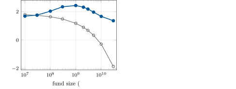
The profit-maximising size is therefore larger than the size that maximises the return on capital, which is the smallest; Berk and Green built a theory of active management on this decreasing return to scale. Figure 28.1 draws chapter 27’s fifty-name book at ten sizes from $10 million to $30 billion, in two versions. The fixed rule (costs ignored, the forecast smoothed over fifty days) trades the same way at every size: its net Sharpe ratio falls from 1.79 at $10 million to 0.34 at $5 billion and at $10 billion, halving at $2.02 billion, and its dollar profit peaks at $3 billion, $146 million a year. The book re-optimised at each size, with the costs inside and a one-day smoothing, peaks at a Sharpe ratio of 2.43 at $1 billion and is still at 1.36 at $30 billion, where its profit, $806 million a year, is still growing: re-optimising at size is the largest single extension of capacity, because it changes how much a book trades as it grows.
rs_capacity.curve.28.2 Alpha decay in production
A strategy’s capacity changes after it goes live, for reasons chapter 13 measured: the signal decays as others find it, and the post-publication decline of published factors is the public record of that. Capacity decays twice over, since the gross return falls and the costs, now shared with the competitors trading the same names, rise. The capacity curve should therefore be redrawn with the live information coefficient and with the costs measured on the firm’s own fills (chapters 23 and 27), and a strategy should be sized below its estimated profit-maximising size, where the curve is flat: the profit lost by being smaller is small, the protection against a curve that has moved is large.
28.3 Detecting crowding
Definition 28.3 (Crowding, crowded trade, comomentum, unwind)
Crowding is the presence of many investors in the same positions; a crowded trade is a position held by enough of them that their joint exit would move prices. Comomentum (Lou and Polk) is the average correlation of the abnormal returns of the stocks a momentum strategy holds, a measure of how many traders act on them. An unwind is the rapid reduction of a crowded position by some of its holders, which moves the prices at which the others mark theirs.
Stein named the problem: for a strategy whose value has no anchor in fundamentals, an arbitrageur cannot know how many of its peers are entering the same trade, and the leverage each chooses in private creates a fire-sale risk for all. Pedersen analysed why traders crowd in and why they run. Three monitors make crowding visible (Listing 28.1): the correlation among the returns of a strategy’s own names, net of the risk model’s factors (comomentum for a momentum book: high values predicted reversals); the overlap of the firm’s book with estimates of others’ books (from regulatory holdings filings, or from the returns of competitors’ products); and short interest and days to cover on the short side (Book 1, chapter 16). None is conclusive, and each is noisy; they belong on the risk dashboard next to the book’s liquidity.
28.4 August 2007
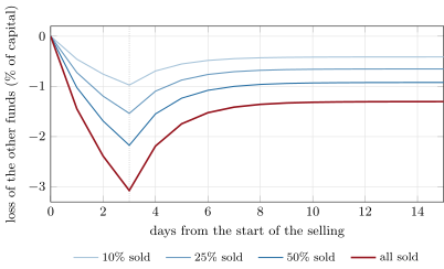
The chapter’s unwind (Listing 28.2) puts five funds of $2 billion each in long–short books of 500 stocks, four times their capital in gross exposure, a hundred names a side; each stock trades $200 million a day with a daily volatility of 2%. Each fund ranks the stocks on a mixture of a common score and its own, with a weight that sets how much their books overlap. One fund sells a fraction of its book over three days. Each day its trades move prices by a square-root impact, 30% of which stays while the rest decays with a half-life of a day, and the other four funds mark their books to the moved prices.
| overlap of the books (cosine) | ||||
| fraction of the book sold | 0.04 | 0.18 | 0.43 | 1.00 |
| 10% | ||||
| 25% | ||||
| 50% | ||||
| 100% | ||||
The table gives the other funds’ peak loss, as a fraction of their capital; it comes on the third day, the last of the selling, in every case. The loss grows in proportion to the overlap and with the square root of the fraction sold, since impact is a square root: selling a quarter of the book costs the others half as much as selling all of it. With identical books and the whole book sold, the others lose 3.07% of their capital without trading, the seller 2.00% (it also pays for its trades). Then the temporary impact decays: by day fifteen the others’ loss is 1.30%, the permanent share (Figure 28.2). The recovery is the Friday of August 2007, and the ones who lost most were those who sold at the bottom, locking in the temporary part. A fund that knows the loss is temporary and has the capital to hold on loses only the permanent part; a fund with a stop-loss becomes the next seller, which is how an unwind spreads.
rs_capacity.unwind.28.5 Tutorial: the week of 6 August 2007
Goal. Draw the capacity curves of chapter 27’s book, find the profit-maximising size and the size at which the net Sharpe ratio halves, and simulate the unwind over a grid of overlaps and fractions sold. End state: the table, Figures 28.1 and 28.2, and the factor returns of August 2007 from data/research/ff_aug2007.csv.
Capacity helpers: the curve, its peak and the size at a fraction of the best.
def capacity_curve(sizes, net_returns, vols) -> dict:
    s, n, v = (np.asarray(a, float) for a in (sizes, net_returns, vols))
    return {"size": s, "net": n, "sr": n / v, "profit": s * n}


def profit_maximising(curve: dict) -> float:
    return float(curve["size"][int(np.argmax(curve["profit"]))])


def size_at_fraction(curve: dict, frac: float = 0.5, key: str = "sr"):
    y, s = np.asarray(curve[key], float), np.log(np.asarray(curve["size"], float))
    target = frac * y.max()
    start = int(np.argmax(y))
    for i in range(start, len(y) - 1):
        if y[i + 1] < target <= y[i]:
            x = s[i] + (target - y[i]) / (y[i + 1] - y[i]) * (s[i + 1] - s[i])
            return float(math.exp(x))
    return None
Listing 28.1. Capacity curve, profit-maximising size and halving size. code/firm/capacity/firm_capacity.py The unwind: trades at the open, square-root impact, permanent and decaying parts, marking.
def unwind(books, capitals, seller: int, fraction: float, days: int, adv, sigma, eta: float = 0.7,
           permanent: float = 0.3, half_life: float = 1.0, horizon: int = 10) -> dict:
    """books (funds, n) weights; capitals (funds,) dollars. The seller trades fraction / days of its book each day for
    `days` days (selling longs, buying back shorts). Day t's impact on stock i is -sign(q) eta sigma_i sqrt(|q| /
    adv_i) for its net dollar trade q; a share `permanent` stays, the rest decays with the half-life (days). Every fund
    holds its book (the seller's shrinking) and marks it to the moved prices."""
    B, K = np.asarray(books, float), np.asarray(capitals, float)
    adv, sigma = np.asarray(adv, float), np.asarray(sigma, float)
    n = B.shape[1]
    decay = 0.5 ** (1.0 / half_life)
    temp, perm = np.zeros(n), np.zeros(n)
    level = np.zeros((horizon + 1, n))
    hold = B.copy()
    pnl = np.zeros((horizon, len(K)))
    for t in range(horizon):
        trade = -B[seller] * fraction / days if t < days else np.zeros(n)
        hold[seller] = hold[seller] + trade                              # trades at the open
        q = trade * K[seller]
        push = np.sign(q) * eta * sigma * np.sqrt(np.abs(q) / adv)
        temp = temp * decay + (1 - permanent) * push
        perm = perm + permanent * push
        level[t + 1] = temp + perm
        move = level[t + 1] - level[t]
        pnl[t] = (hold * move).sum(axis=1)
        pnl[t, seller] -= float(np.abs(trade) @ np.abs(push)) / 2          # it traded through its own move
    return {"price": level, "pnl": pnl, "cum": np.cumsum(pnl, axis=0)}
Listing 28.2. Funds marking overlapping books while one sells. code/firm/capacity/firm_capacity.py - Run
rs_capacity.curve,summary,unwind(theta, fraction),fig_capacity.py, andrs_fetch_aug2007.pyonce.
What to change next. Give the non-selling funds a stop-loss at 1% and let them sell when it is hit: the cascade; make the permanent share depend on whether market makers stay (Khandani and Lo’s withdrawal of capital).
28.6 Build: capacity and crowding
Purpose. Every strategy is sized from its capacity curve and monitored for crowding; the risk of an unwind by others is a scenario in the firm’s stress tests.
Interface. capacity_curve(sizes, net_returns, vols), profit_maximising(curve), size_at_fraction(curve, frac, key), avg_pairwise_corr(R), comomentum(R_long, R_short), overlap(w1, w2), unwind(books, capitals, seller, fraction, days, adv, sigma, eta, permanent, half_life, horizon).
Rules. Capacity curves are drawn from backtests re-run at each size with the firm’s fitted costs, and redrawn with live information coefficients; a strategy runs below its profit-maximising size; crowding monitors are reviewed with the book’s liquidity.
Acceptance tests. code/firm/capacity/tests/: the profit-maximising and halving sizes of a strategy with square-root costs against their closed forms; pairwise correlation and comomentum of a planted common factor; overlap by hand; an unwind in which the same book loses and the opposite book gains the same, temporary impact that comes back, and permanent impact that does not.
Stretch. Cascades with stop-losses; crowding estimated from regulatory holdings filings; capacity shared among the firm’s strategies.
Sources and further reading
- A. E. Khandani and A. W. Lo, “What happened to the quants in August 2007? Evidence from factors and transactions data”, Journal of Financial Markets 14(1), 2011.
- D. Lou and C. Polk, “Comomentum: inferring arbitrage activity from return correlations”, Review of Financial Studies 35(7), 2022.
- L. H. Pedersen, “When everyone runs for the exit”, NBER Working Paper 15297, 2009.
- J. C. Stein, “Presidential address: sophisticated investors and market efficiency”, Journal of Finance 64(4), 2009.
- J. B. Berk and R. C. Green, “Mutual fund flows and performance in rational markets”, Journal of Political Economy 112(6), 2004.
- K. R. French, Data Library, Fama/French 3 Factors and Momentum Factor (daily).
28.7 Exercises
Exercise 28.1 ★
A strategy earns 10% a year gross and its costs reach 10% at $10 billion, growing as the square root of size. Find its profit-maximising size and its net return there.
Solution
Solution of Exercise 28.1.
gives ; billion, where the net return is .
Exercise 28.2 ★
Why is the profit-maximising size larger than the size that maximises the return on capital?
Solution
Solution of Exercise 28.2.
The return on capital falls from the first dollar, but the dollar profit is size times return: it keeps rising while the return falls more slowly than size grows, up to the point where the marginal dollar earns nothing ().
Exercise 28.3 ★
In the chapter’s unwind with identical books, how large is one day’s price push on a long name when the whole book is sold over three days?
Solution
Solution of Exercise 28.3.
A position of 2% of $2 billion, $40 million, sold over three days: $13.3 million a day against $200 million traded, 6.7% of volume. The push is a day.
Exercise 28.4 ★★
Why does the other funds’ loss grow with the square root of the fraction sold, and in proportion to the overlap?
Solution
Solution of Exercise 28.4.
Each name’s push is proportional to the square root of the seller’s trade in it, and the trade is proportional to the fraction sold: the loss of a fund holding the same name scales as its square root. A non-seller’s loss is its book times the push, so it is proportional to how much of its book lies where the seller trades: the overlap.
Exercise 28.5 ★★
In the week of 6 August 2007 the market rose while value and momentum fell by ten standard deviations. What does that say about who was trading?
Solution
Solution of Exercise 28.5.
The loss was confined to long–short factor books, not the market: someone was selling the long side and buying back the short side of value and momentum books at the same time. That is the signature of deleveraging by funds holding similar books, as Khandani and Lo concluded, not of news.
Exercise 28.6 ★★
Why does re-optimising at each size extend capacity so much more than any change to the signal?
Solution
Solution of Exercise 28.6.
Costs grow faster than size, so the damage of size comes from trading. A book re-optimised at each size trades less as it grows (at $10 billion it turns over 1.8% of capital a day against 227% at $10 million in chapter 27), which keeps its costs from outrunning its return; the signal was the same.
Exercise 28.7 ★★★
Coding. With rs_capacity.unwind, compare the other funds’ loss at day fifteen with their peak loss, and relate the ratio to the permanent share.
Solution
Solution of Exercise 28.7.
With identical books, day fifteen over the peak is for the whole book and for a tenth: above the permanent share of 0.3 because the peak, on the third day, already includes some decay of the first days’ temporary impact.
Exercise 28.8 ★★★
Find the flaw. “Our strategy’s capacity is $5 billion: at that size its backtest still has a Sharpe ratio of 0.34 after costs.”
Solution
Solution of Exercise 28.8.
A positive Sharpe ratio is not a capacity: at $5 billion the fixed rule’s ratio has fallen to a fifth of its best (0.34 against 1.79) and its dollar profit is past its peak ($146 million at $3 billion, $122 million at $5 billion). By the chapter’s criterion its capacity is $2.02 billion, and the estimate is itself uncertain; run it below that.
28.8 Problem: The Week of 6 August 2007
Problem 28.1
Weekend problem — how big, and with whom
Chapter 27’s book at many sizes, and the chapter’s unwind.
Part I — Capacity.
- State and prove the profit-maximising size under square-root costs.
- Give the fixed rule’s net Sharpe ratio from $10 million to $30 billion.
- Where does its profit peak, and where does its Sharpe ratio halve?
- What does re-optimising at each size change?
- How would you size the strategy, and why below its profit-maximising size?
Part II — Decay and crowding.
- Why does capacity decay after a strategy goes live?
- What are Stein’s two complications?
- What is comomentum, and what did high values predict?
- Which monitors would you put on the dashboard?
Part III — The unwind.
- Describe the simulated funds and the impact model.
- Give the other funds’ peak losses over the grid.
- When does the peak come, and what remains at day fifteen?
- What did the value and momentum factors do from 6 to 10 August 2007?
- What did Khandani and Lo identify?
Part IV — The verdict.
- State the named result: the peak loss of the non-selling funds against the fraction of the overlapping book sold, and the size at which the strategy’s net Sharpe ratio halves.
- What should a fund do on the third day of an unwind it did not start?
- How would stop-losses change the table?
- How does the firm’s own set of strategies crowd itself (chapter 27’s netting)?
- What would you ask a new strategy’s author about capacity?
- In one sentence: what determines a strategy’s capacity?
Solution
Solution of Problem 28.1.
- , where ; the net return there is .
- 1.79, 1.74, 1.64, 1.48, 1.18, 0.90, 0.68, 0.34, , at $10m, $30m, $100m, $300m, $1bn, $2bn, $3bn, $5bn, $10bn, $30bn.
- Profit peaks at $3 billion ($146 million a year); the Sharpe ratio halves at $2.02 billion.
- The book trades less as it grows: Sharpe ratio 2.43 at $1 billion, 1.36 at $30 billion, with profit still growing ($806 million).
- Below the profit-maximising size, where the curve is flat, because the curve will move (decay, competitors) and the estimate is uncertain.
- The signal decays as others find it, and the costs rise as others trade the same names.
- Crowding (an arbitrageur cannot know how many peers are in the same trade) and leverage (a private choice that creates a fire-sale externality).
- The average abnormal return correlation among a momentum strategy’s stocks; high values predicted strong reversals of momentum returns.
- Correlation among the strategy’s own names net of factors, overlap with estimated books of others, short interest and days to cover, and the book’s liquidity.
- Five funds of $2 billion, gross four times capital, 100 names a side from 500 stocks trading $200 million a day at 2% volatility; one sells over three days; square-root impact with , 30% permanent, the rest decaying with a half-life of one day.
- From (10% sold, overlap 0.04) to (all sold, identical books); the table in the text.
- On the third day, the last of the selling; at day fifteen the whole-book case has recovered to .
- From 6 to 9 August value fell 2.28% and momentum 3.43% (10.6 and 12.5 daily standard deviations) while the market rose 1.39%; on 10 August value regained 1.42% and momentum 1.15%.
- Losses of long–short value-type books that began in July, two unwinds on 1 and 6 August starting with financials, long book-to-market and short momentum, and a withdrawal of market-making capital from 8 August.
- Named result. With identical books, the non-selling funds’ peak loss is 0.97%, 1.54%, 2.17% and 3.07% of capital when a tenth, a quarter, half and all of the book is sold (proportionally less at lower overlap); the fixed rule’s net Sharpe ratio halves at $2.02 billion.
- Not sell at the bottom if it can hold: the temporary part comes back; reduce only as much as its own limits require, and provide liquidity if it has capital.
- They turn losses into more selling: the peaks deepen and spread to funds that did not overlap with the first seller.
- Its strategies’ trades in the same names add up under a concave cost law, so their combined capacity is less than the sum.
- The capacity curve at the firm’s costs, the turnover and holding period, the names’ liquidity, and who else is likely to hold the same book.
- Its costs as it grows, set by how much it trades in which names, and the other capital in the same trade.
28.9 Interview questions
Interview question 28.1 ★ researcher, risk
What happened to quantitative equity funds in August 2007?
Solution
Solution of Interview question 28.1.
In the week of 6 August 2007 long–short quantitative equity books lost heavily with no news, as value and momentum factors fell by ten or more daily standard deviations while the market rose; on 10 August much of it came back. Khandani and Lo attribute it to the unwinding of similar books by several funds and a withdrawal of market-making capital.
Interview question 28.2 ★★ researcher
How do you estimate a strategy’s capacity?
Solution
Solution of Interview question 28.2.
Re-run the backtest at a grid of sizes with the firm’s fitted cost model (spread and square-root impact), re-optimised at each size; read the net Sharpe ratio and dollar profit against size; take the profit-maximising size and a criterion such as the size at which the net Sharpe ratio halves; redraw with live data.
Interview question 28.3 ★★ researcher, risk
How would you tell whether your strategy is crowded?
Solution
Solution of Interview question 28.3.
Look for excess correlation among the strategy’s names net of risk-model factors (comomentum), overlap with estimated books of others (holdings filings, returns of similar products), high short interest and days to cover on the short side, and whether the strategy’s losses coincide with others’.
Interview question 28.4 ★★ risk
Another fund with a book like yours is liquidating. What do you do?
Solution
Solution of Interview question 28.4.
Estimate the overlap and the seller’s size; expect a temporary loss on the overlapping part; do not sell into it unless limits force you; reduce the most illiquid overlapping positions early if you must; consider providing liquidity to the seller if the permanent part is small.
Interview question 28.5 ★★ researcher, trader
Why can a strategy’s dollar profit keep rising after its Sharpe ratio has started to fall?
Solution
Solution of Interview question 28.5.
Profit is size times net return: the return (and the Sharpe ratio) falls from the first dollar under concave costs, but profit rises while size grows faster than the return falls, up to .
Interview question 28.6 ★★★ researcher
Model the loss of a fund that holds a book overlapping a seller’s, with square-root impact and a permanent share, and derive how it scales with the fraction sold.
Solution
Solution of Interview question 28.6.
If the seller trades of each name over a day and the push is , a fund holding of the name loses on the day, of which the permanent share stays; spreading the sale over days and letting the rest decay gives the chapter’s paths.