Research Craft: Predictors, Backtests, Measurement, Portfolios · Research

6Anatomy of a Predictor

Two researchers report the information coefficient of the same reversal signal on the same stocks: 0.038 and 0.007. Both computed a rank correlation between minus a past return and a future return, and both computed it correctly. The first correlated yesterday’s return with tomorrow’s; the second the last five days’ return with the next five days’. A predictor is not a formula: it is a formula, a target, a horizon, a normalisation and a neutralisation, and a number describing it means nothing without all five. This chapter takes a predictor apart into those pieces, measures it with the information coefficient and the standard errors that the measurement needs, and ends with the predictor card, the one-page record that the rest of Part II fills for every predictor it studies. Its data are the book’s synthetic market (chapter 5), whose one-day reversal is known to be real.

6.1 The target

Definition 6.1 (Predictor, prediction target, forecast horizon)

A predictor is a number computed for each security at a decision time from data known at that time, intended to be correlated across securities with a later quantity, its prediction target (usually a return). The forecast horizon is the span of the target: the return over the next day, the next five days, the next month.

Figure 6.1. The timing of a predictor. Everything it uses is known at the close of the decision day

t

; its target begins the next day. A predictor whose window reaches past

t

, or a target that starts at

t

, has look-ahead (chapter 3).

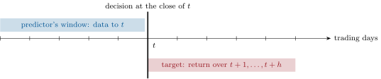
The horizon is part of the predictor. On the synthetic market, reversal measured four ways gives four different numbers: minus the last day’s return has a mean rank IC of 0.0385 with the next day’s return ( $t = 17.8$ ), and 0.0162 with the next five days’ return; minus the last five days’ return has 0.0187 with the next day and 0.0074 with the next five ( $t = 2.4$ ). The simulator plants a reversal of one day, and every measurement that dilutes that day, on either side, sees less of it. A real predictor’s horizon is unknown and must be found (chapter 13), but the lesson carries: the pair (predictor window, target horizon) is what is measured.

Definition 6.2 (Residual return)

The residual return of a security over a period is its return minus the part explained by chosen factor exposures, estimated on each date by a cross-sectional regression of the returns on the exposures: what is left after the market, the industries or the styles.

Three targets are common: the raw return, the return in excess of a market (or benchmark), and a residual return. For a rank IC across securities on one date the first two are the same, since subtracting one number from every return leaves their ranks unchanged: on the synthetic market both give 0.0074 for the five-day reversal. The residual is different, and the next section says when it matters.

6.2 Normalisation

Definition 6.3 (Cross-sectional z-score, rank transform)

The cross-sectional z-score of a predictor on a date is its value minus that date’s mean across securities, divided by that date’s standard deviation, usually clipped at a few units. Its rank transform replaces each value by its rank on the date, scaled to lie in $(-\tfrac12, \tfrac12)$ .

Raw predictors are not comparable across dates (a five-day return of 3% is large in a calm week and small in a crash) or across predictors (a return and a ratio of book value to price have different units). Normalising each date’s cross-section removes both problems and turns a predictor into a set of relative bets, which is what a market-neutral book holds. The z-score keeps the shape of the distribution and must be clipped (or the predictor winsorised, Book 4, chapter 15), because one extreme name otherwise dominates the date. The rank transform discards the shape entirely: it is robust, and the rank IC, Spearman’s correlation of Book 4, chapter 15, is the Pearson correlation of two rank-transformed variables. Nothing is free: the rank transform treats the difference between the first and second names like that between the 500th and the 501st.

6.3 Neutralisation

Definition 6.4 (Neutralisation)

Neutralisation is the removal from a predictor, or from a target, of its component along chosen exposures, by taking on each date the residual of a cross-sectional regression on them: industry neutralisation removes industry means, beta neutralisation the component along market beta.

Proposition 6.5 (What neutralising the target does to the IC)

On one date, write the target as $y = f + u$ , where $f$ is its projection on the exposures and $u$ the residual, uncorrelated with $f$ . If the predictor $s$ is uncorrelated with $f$ , then

\operatorname{corr}(s, u) = \operatorname{corr}(s, y)\,\sqrt{\frac{\Var(y)}{\Var(u)}}.

Proof. $\Cov(s, y) = \Cov(s, u)$ , since $s$ is uncorrelated with $f$ . Divide by $\sqrt{\Var(s)\Var(y)}$ and by $\sqrt{\Var(s)\Var(u)}$ in turn. ∎

If the exposures explain a share $1 - \rho$ of the target’s cross-sectional variance, measuring against the residual raises the IC by $1/\sqrt\rho$ : the predictor was right about the part it could see, and the factor part was noise to it. In the default synthetic market the market beta and ten industries explain only 10% of the variance of five-day returns across stocks, and neutralising changes the five-day reversal’s IC from 0.0074 to 0.0064, within noise. In a variant whose industries move more (30% volatility a year instead of 8%) they explain 52%, and the proposition predicts a ratio of $1/\sqrt{0.476} = 1.45$ : the IC goes from 0.0043 to 0.0067 against the residual target, and to 0.0086 when the predictor is industry-neutralised too, with the $t$ -statistic going from 0.8 to 3.5 (Figure 6.2). Neutralising the predictor removes its own industry component, which in this market carries no information about the future.

Five-day reversal against five-day returns in a synthetic market whose industries move strongly (30% a year): raw predictor and raw target, raw predictor and residual target, industry-neutral predictor and residual target. Labels are the HAC t-statistics. Data: firm.synthmkt with ind_vol=0.30, seed 1. — **Figure 6.2.** Five-day reversal against five-day returns in a synthetic market whose industries move strongly (30% a year): raw predictor and raw target, raw predictor and residual target, industry-neutral predictor and residual target. Labels are the HAC $t$ -statistics. 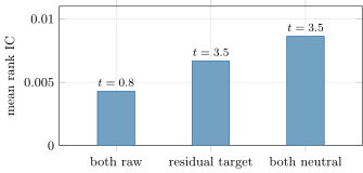Data: `firm.synthmkt` with `ind_vol=0.30`, seed 1.

6.4 The information coefficient and its standard error

Definition 6.6 (Information coefficient, rank information coefficient)

The information coefficient (IC) of a predictor on a date is the correlation, across the securities of that date, between the predictor and its target. The rank information coefficient is the same with ranks (Spearman’s correlation). A predictor is summarised by the time series of its ICs: their mean, their standard deviation, and the ratio of the two.

Definition 6.7 (IC information ratio, quantile spread)

The IC information ratio (ICIR) is the mean IC divided by its standard deviation over dates, annualised by $\sqrt{252/h}$ for an $h$ -day horizon sampled every $h$ days. The quantile spread is the mean target of the securities in the predictor’s top quantile minus that of the bottom quantile, date by date.

Two facts about the IC’s noise decide how long a predictor must be observed. On one date with $N$ names and no predictability, the IC has a standard deviation of about $1/\sqrt{N - 1}$ (0.032 for 1 000 names); a mean IC of 0.01 is therefore invisible on any single date and must be accumulated over hundreds. And when the target spans $h$ days but the IC is computed every day, the targets of consecutive dates share $h - 1$ days, the ICs are strongly autocorrelated, and the naive standard error of their mean is too small.

Proposition 6.8 (Overlapping targets)

If the daily IC series of an $h$ -day target has autocorrelations $\rho_k$ that decline linearly to zero at lag $h$ (as for a persistent predictor and non-overlapping daily returns), the variance of its mean over $n$ dates is approximately $h$ times the naive $\Var/n$ : the naive $t$ -statistic overstates by up to $\sqrt h$ . The Newey–West estimator with $h - 1$ lags (Book 4, chapter 11) corrects it, and so does using every $h$ -th date.

Proof. $\Var(\bar x) \approx \frac{\sigma^2}{n}\bigl(1 + 2\sum_{k=1}^{h-1}\rho_k\bigr)$ with $\rho_k = 1 - k/h$ ; the sum is $(h - 1)/2$ , so the bracket is $h$ . ∎

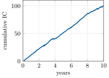
For the five-day reversal against five-day targets, the naive $t$ -statistic is 3.85 and the corrected one 2.39: the ratio 1.61 is below $\sqrt5 = 2.24$ because the reversal is not persistent. Using only every fifth date gives 1.31, a valid but less efficient estimate from a fifth of the data. For the one-day reversal against one-day returns there is no overlap: 0.0385, $t = 17.8$ , an annualised ICIR of 6.4 once the predictor is neutralised, a number no real daily predictor reaches after costs; the simulator plants it strongly so that later chapters’ tools have something to find.

The one-day reversal on the synthetic market. Left: its rank IC with the return of each of the next ten days; the information is spent on the first day (0.0385), the second has 0.0008. Right: the cumulative sum of its daily IC over ten years, neutralised to beta and industries; a straight line is a stable predictor. Data: firm.synthmkt, seed 1. — **Figure 6.3.** The one-day reversal on the synthetic market. Left: its rank IC with the return of each of the next ten days; the information is spent on the first day (0.0385), the second has 0.0008. Right: the cumulative sum of its daily IC over ten years, neutralised to beta and industries; a straight line is a stable predictor. Data: `firm.synthmkt`, seed 1.

6.5 The predictor card

Definition 6.9 (Predictor card)

A predictor card is the one-page record of a predictor: its definition as a formula; its inputs and the knowledge time of each; its rationale; its horizon and measured half-life; its normalisation and neutralisation; its known failure modes; its sources. The measured statistics come from a tested script, never from memory.

The card is the unit in which Part II of this book, and a research group, accumulates knowledge: a predictor without a card has not been studied, only tried. Its fields force the questions of this chapter to be answered before the predictor is used. Here is the first.

Predictor card 6.1 — One-day reversal

Definition. $s_{i,t} = -r_{i,t}$ , the day’s return with the sign changed, ranked across the universe and neutralised to market beta and industries.

Inputs and timestamps. The closes of days $t-1$ and $t$ , known at the close of $t$ ; betas and industries as of $t$ .

Rationale. Liquidity providers are paid, through a reversal, for absorbing demand for immediacy (chapter 1).

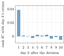
Horizon and half-life. One day. On the synthetic market the rank IC is 0.0385 with day $t+1$ and 0.0008 with day $t+2$ : the half-life is under a day.

Normalisation. Cross-sectional rank; residual on beta and industry dummies. Neutralised, its mean rank IC is 0.040 with an annualised ICIR of 6.4 ( $t = 20.1$ ) on the synthetic market, which plants it.

Failure modes. Moves on news (earnings days) do not revert; the daily turnover costs more than the IC earns in liquid large stocks; crowding by many liquidity providers.

Sources. N. Jegadeesh (1990); B. N. Lehmann (1990); rs_anatomy.card() for the numbers.

6.6 Tutorial: measuring a predictor

Goal. Measure reversal on the synthetic market with every choice of this chapter made explicitly, and fill its card. End state: Figures 6.2 and 6.3; the horizon table; the $t$ -statistics 3.85 (naive) and 2.39 (corrected); Predictor card 6.1.

Neutralise. A cross-sectional regression per date on a constant and the exposures; names with a missing value are skipped, not filled.

def residualise(y: np.ndarray, X: np.ndarray) -> np.ndarray:
    """Per date, the residual of y on a constant and the exposures (names with any missing value are skipped)."""
    y = np.asarray(y, float)
    out = np.full(y.shape, np.nan)
    for t in range(y.shape[0]):
        Xt = X[t] if X.ndim == 3 else X
        Xt = np.column_stack([np.ones(y.shape[1]), Xt])
        ok = ~np.isnan(y[t]) & ~np.isnan(Xt).any(axis=1)
        if ok.sum() <= Xt.shape[1] + 1:
            continue
        b = np.linalg.lstsq(Xt[ok], y[t, ok], rcond=None)[0]
        out[t, ok] = y[t, ok] - Xt[ok] @ b
    return out

Listing 6.1. Per-date residuals on the exposures. code/firm/predictor/firm_predictor.py

Summarise. The IC series’ mean, its information ratio and two $t$ -statistics, the second with $h - 1$ Newey–West lags for overlapping targets.

def ic_summary(ic, h: int = 1, periods: int = 252) -> dict:
    """Mean IC and its t-statistics: naive (as if the dates were independent) and Newey-West with h - 1 lags,
    the right correction when h-day targets overlap on consecutive dates. The IC information ratio is the mean
    over the standard deviation; its annual version scales by sqrt(periods / h)."""
    x = np.asarray(ic, float)
    x = x[~np.isnan(x)]
    n = len(x)
    mean, sd = float(x.mean()), float(x.std(ddof=1))
    se_naive = sd / math.sqrt(n)
    se_hac = math.sqrt(long_run_variance(x, max(0, h - 1)) / n) if h > 1 else se_naive
    return {"mean": mean, "sd": sd, "icir": mean / sd, "icir_annual": mean / sd * math.sqrt(periods / h),
            "t_naive": mean / se_naive, "t_hac": mean / se_hac, "n": n}

Listing 6.2. The IC summary. code/firm/predictor/firm_predictor.py

Run horizon_ics(), study() and card(); then neutralisation on a market simulated with ind_vol=0.30, and fig_anatomy.py.

What to change next. Replace the rank transform by a z-score clipped at 3, then at 10, and watch the IC’s standard deviation; neutralise to the size exposure as well and check that the reversal survives.

6.7 Build: the predictor toolkit

Purpose. One implementation of targets, normalisers, neutralisation and the IC for every predictor of the book, so that numbers from different chapters (and, later, Books 8 and 9) are comparable.

Interface. forward_return(ret, h), excess(target, market), residualise(y, X) and neutralise, zscore(x, clip), rank_transform(x), ic_series(signal, target, method), ic_summary(ic, h, periods), quantile_spread(signal, target, q), PredictorCard.

Rules. Panels are (dates, names) with NaN for absent names; a predictor at row $t$ is known at the close of $t$ and its target starts at $t+1$ ; missing values are skipped per date, never imputed; a date with fewer than 20 names has no IC.

Acceptance tests. code/firm/predictor/tests/: compounding and gaps in forward returns; clipping and ranks; residuals orthogonal to the exposures; an IC of 0.05 recovered with the $1/\sqrt N$ noise; a naive $t$ more than 2.5 times the HAC $t$ for a persistent predictor and overlapping 20-day targets; a card’s fields.

Stretch. Weighted ICs (by liquidity); ICs by group (industry, size bucket); a bootstrap of the IC’s mean over dates.

Sources and further reading

R. C. Grinold and R. N. Kahn, Active Portfolio Management, 2nd ed., McGraw-Hill, 2000.
E. E. Qian, R. H. Hua and E. H. Sorensen, Quantitative Equity Portfolio Management, Chapman & Hall/CRC, 2007.
W. K. Newey and K. D. West, “A simple, positive semi-definite, heteroskedasticity and autocorrelation consistent covariance matrix”, Econometrica 55(3), 1987.
N. Jegadeesh, “Evidence of predictable behavior of security returns”, Journal of Finance 45(3), 1990; B. N. Lehmann, “Fads, martingales, and market efficiency”, Quarterly Journal of Economics 105(1), 1990.

6.8 Exercises

Exercise 6.1 ★

A universe has 800 names. What is the standard deviation of a single date’s IC for a useless predictor, and how many independent dates are needed for a mean IC of 0.01 to reach $t = 2$ ?

Solution

Solution of Exercise 6.1.

$1/\sqrt{799} = 0.0354$ . A mean of 0.01 reaches $t = 2$ when $0.01\sqrt n/0.0354 = 2$ , $n = 50$ independent dates, if the only noise were the cross-sectional sampling; common shocks make real IC series noisier, and several times as many dates are needed in practice.

Exercise 6.2 ★

A predictor’s daily rank IC against the next day’s raw return is 0.02. What is its rank IC against the next day’s return in excess of the equal-weighted market? And against the return in excess of each stock’s own beta times the market?

Solution

Solution of Exercise 6.2.

Still 0.02 against the market-excess return: subtracting one number from every return leaves the ranks unchanged. Against beta-adjusted returns it changes whenever betas differ, because each stock subtracts a different amount; how much depends on how the predictor correlates with beta.

Exercise 6.3 ★

A daily IC series has mean 0.012 and standard deviation 0.08. What is the annualised ICIR?

Solution

Solution of Exercise 6.3.

$0.012/0.08 \times \sqrt{252} = 2.38$ .

Exercise 6.4 ★★

Industry factors explain 40% of the cross-sectional variance of monthly returns, and a stock-selection predictor with no industry content has an IC of 0.03 against raw returns. What IC should it show against industry-residual returns?

Solution

Solution of Exercise 6.4.

The residual keeps $\rho = 0.6$ of the variance: $0.03/\sqrt{0.6} = 0.039$ .

Exercise 6.5 ★★

A 20-day target is scored every day for a very persistent predictor. By the proposition, by how much can the naive $t$ -statistic overstate? What $t$ does a naive 6.0 correspond to?

Solution

Solution of Exercise 6.5.

Up to $\sqrt{20} = 4.47$ ; a naive 6.0 may be as little as $6.0/4.47 = 1.34$ .

Exercise 6.6 ★★

Give one reason to prefer a rank IC to a Pearson IC and one reason to prefer the Pearson IC, in terms of what a portfolio built from the predictor earns.

Solution

Solution of Exercise 6.6.

Rank IC: robust to outliers in the predictor and in returns, so one extreme name does not decide a date. Pearson IC: a portfolio whose weights are proportional to the predictor earns in proportion to the Pearson correlation, magnitudes included, so it measures what a linear book would make.

Exercise 6.7 ★★★

Coding. With ic_series and ic_summary, measure the one-day reversal against the next day’s return separately on days when the market’s absolute return was in its top decile and on the other days. Which days carry the predictor?

Solution

Solution of Exercise 6.7.

On the tenth of days with the largest absolute market return the rank IC is 0.037 ( $t = 5.0$ ); on the others 0.039 ( $t = 17.1$ ). The reversal is carried evenly: the simulator reverses a fixed share of each day’s specific shock, whatever the market does. On real data this is the kind of dependence to test, not to assume.

Exercise 6.8 ★★★

Find the flaw. “Our 60-day predictor has a mean IC of 0.04 against 60-day forward returns, computed daily over five years: 1 260 dates, so $t = 0.04/(0.10/\sqrt{1\,260}) = 14$ .”

Solution

Solution of Exercise 6.8.

The 60-day targets of consecutive days overlap by 59 days, so the 1 260 ICs are nowhere near independent: there are about 21 non-overlapping periods. The proposition bounds the overstatement at $\sqrt{60}$ : the honest $t$ may be as low as $14/7.75 = 1.8$ . Use Newey–West with 59 lags, or every 60th date.

6.9 Problem: Two ICs for One Signal

Problem 6.1

Weekend problem — what the choices of a measurement do to a predictor’s numbers

The synthetic market with its default configuration (1 000 names, ten years, seed 1), and a variant with industry volatility of 30% a year. The predictor is reversal: minus a past return.

Part I — Horizon.

What is the rank IC of one-day reversal against the next day’s return, and its $t$ -statistic?
And of five-day reversal against the next five days’ return?
What are the two mixed pairs (one-day against five, five-day against one)?
Which of the four is the planted effect, and why are the others smaller?
What is the one-day reversal’s IC with the return of the second day after the decision?

Part II — Targets and neutralisation.

Why do the raw and the market-excess targets give the same rank IC?
What share of five-day return variance do beta and industries explain in the default market?
In the strong-industry variant, what share, and what ratio does the proposition predict?
What are the three ICs of Figure 6.2 and their $t$ -statistics?
Why does neutralising the predictor add to neutralising the target?

Part III — Standard errors.

What are the naive and corrected $t$ -statistics of the five-day reversal against five-day targets?
Why is their ratio below $\sqrt5$ ?
What does using every fifth date give, and why is it lower still?
What is the standard deviation of one date’s IC with 1 000 names and no predictability?

Part IV — The card.

What are the card’s mean IC, annualised ICIR and $t$ -statistic?
What does the card say about the half-life, and from which numbers?
Which field of the card would change first if the market’s liquidity providers became more numerous?
State the named result: the five-day reversal’s naive and HAC $t$ -statistics for overlapping targets, and the IC gained by neutralising target and predictor in the strong-industry market.
What should a research report say when it quotes an IC?
In one sentence: what is a predictor?

Solution

Solution of Problem 6.1.

1. 0.0385, $t = 17.8$ . 2. 0.0074, $t = 2.4$ . 3. 0.0162 (one-day against five) and 0.0187 (five-day against one). 4. One-day against one day: the simulator reverses a share of each day’s specific shock the next day, and each other pair adds four days of unrelated returns to the predictor or to the target. 5. 0.0008: nothing. 6. Ranks do not change when one number is subtracted from every return. 7. 10% (the residual keeps 90%). 8. 52%; $1/\sqrt{0.476} = 1.45$ . 9. 0.0043 ( $t = 0.8$ ), 0.0067 ( $t = 3.5$ ), 0.0086 ( $t = 3.5$ ). 10. The predictor’s own industry component carries no information about the future in this market, so removing it removes noise from the predictor as the target’s residual removes noise from the target. 11. 3.85 and 2.39. 12. The bound $\sqrt h$ holds for a persistent predictor; reversal changes daily, so the ICs of consecutive dates overlap less. 13. $t = 1.31$ : valid, but from a fifth of the dates. 14. $1/\sqrt{999} = 0.032$ . 15. 0.040, 6.4, 20.1. 16. Under a day: the IC is 0.0385 with day $t+1$ and 0.0008 with day $t+2$ . 17. The failure modes and then the IC itself: more liquidity providers compete the reversal away (crowding, chapter 28). 18. Named result: for five-day reversal scored daily against overlapping five-day targets the naive $t$ is 3.85 and the HAC $t$ 2.39; in the strong-industry market, neutralising the target and the predictor raises the IC from 0.0043 to 0.0086 and its $t$ from 0.8 to 3.5. 19. The predictor’s formula and window, the target and its horizon, the normalisation and neutralisation, the universe and period, the IC type, and the standard error used. 20. A formula with a target, a horizon, a normalisation and a neutralisation, of which the formula is the least informative part.

6.10 Interview questions

Interview question 6.1 ★ researcher

What is an information coefficient, and what values are good?

Solution

Solution of Interview question 6.1.

The cross-sectional correlation between a predictor and the return it predicts, computed per date and averaged. For stock returns a mean IC of 0.02 to 0.05 is good if it is stable; the information ratio of the IC series and its persistence matter as much as its mean.

What the interviewer is looking for: a definition per date, realistic magnitudes, and attention to stability.

Interview question 6.2 ★★ researcher, mle

You compute a 20-day predictor’s IC every day and get $t = 8$ . Do you believe it?

Solution

Solution of Interview question 6.2.

Not as stated: consecutive 20-day targets overlap by 19 days, so the naive $t$ can overstate by up to $\sqrt{20} = 4.5$ ; $t = 8$ may be about 1.8. Recompute with Newey–West (19 lags) or every 20th date.

What the interviewer is looking for: the overlap correction with a number.

Interview question 6.3 ★★ researcher

Why neutralise a predictor to industries? When would you not?

Solution

Solution of Interview question 6.3.

To remove a component that carries no information but adds noise (industry moves), and to avoid a book that is really an industry bet. Not when the predictor’s information is at the industry level (industry momentum), or when the book is meant to take industry risk.

What the interviewer is looking for: neutralisation as a statement about where the information is.

Interview question 6.4 ★★ researcher, trader

A predictor has an IC of 0.05 against raw returns and 0.02 against residual returns. What is going on?

Solution

Solution of Interview question 6.4.

Most of its apparent power comes from its correlation with the factors that were removed (industry, beta, size): it is partly a factor bet. The 0.02 is its stock-specific skill; whether the rest is worth having depends on whether that factor exposure is rewarded and wanted.

What the interviewer is looking for: the decomposition into factor and specific parts.

Interview question 6.5 ★★ mle, researcher

Rank IC or Pearson IC for a machine-learned return forecast? Why?

Solution

Solution of Interview question 6.5.

Pearson, if positions will be proportional to the forecast (the magnitudes matter), checked alongside the rank IC for robustness; rank if the forecast is used only to order names or if its tails are unreliable.

What the interviewer is looking for: the link between the metric and how the forecast is used.

Interview question 6.6 ★★★ researcher

Derive the standard deviation of a single date’s IC under no predictability, and use it to size the history needed to detect a mean IC of 0.02.

Solution

Solution of Interview question 6.6.

Under no predictability and independent names, the sample correlation of $N$ pairs has variance about $1/(N - 1)$ . The mean of $n$ independent dates has standard error $1/\sqrt{n(N - 1)}$ ; $t = 2$ for a mean of 0.02 with $N = 1\,000$ needs $n = (2/(0.02 \times 31.6))^2 = 10$ dates in theory, but common shocks make the IC’s true dispersion several times larger, and in practice hundreds of dates are needed.

What the interviewer is looking for: the $1/\sqrt{N-1}$ result and awareness that it understates real noise.

Terms defined in this chapter

See all 2333 terms in the glossary