Research Craft: Predictors, Backtests, Measurement, Portfolios · Research

22Performance Measurement

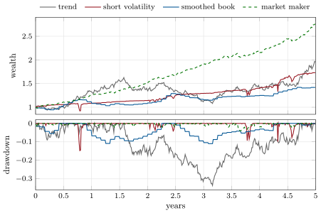
Two strategies have Sharpe ratios of 1.00 and 1.09 over five years of daily returns. The first lost 33.6 per cent peak to trough and spent 791 trading days, more than three years, under water. The second sells out-of-the-money puts and never had a losing quarter; its worst drawdown was 14.8 per cent. Both histories were drawn from the chapter’s simulations, of strategies with long-run volatilities of 15 and 17 per cent, and the second was chosen among the 9% of its simulated five-year histories without a losing quarter. Over the next five years the first has a 14% chance of a drawdown of 30 per cent or more, the second 41%. The Sharpe ratio is the right first number and a dangerous last one. This chapter builds the rest of the tear sheet (standard errors, drawdowns, turnover, the shape of outcomes, the benchmark) as firm.perf, which reads the BacktestResult of chapters 16 to 18, and reads it for four synthetic streams and chapter 16’s momentum book.

22.1 The Sharpe ratio and its standard error

The Sharpe ratio (Book 4, chapter 11) is the mean excess return over its standard deviation; Sharpe introduced it in 1966 as the reward-to-variability ratio and gave it its present name in 1994.

Definition 22.1 (Annualisation)

Annualisation converts a statistic measured on periods of one length to a year: with $q$ periods a year, the mean is multiplied by $q$ , the volatility by $\sqrt q$ and the Sharpe ratio by $\sqrt q$ . The scaling of the volatility and of the Sharpe ratio holds only when the returns are serially uncorrelated.

The standard error of an estimated Sharpe ratio, for independent normal returns, is about $\sqrt{(1 + \mathrm{SR}^2/2)/T}$ per period over $T$ periods (Lo, 2002; Book 4, chapter 11). Annualised, this is nearly $\sqrt{q/T}$ : the length of the history in years sets it, not the frequency. Five years of daily returns give a standard error of 0.45, whatever the strategy; a measured Sharpe ratio of 1.0 has a 95% interval from 0.12 to 1.88. The four five-year streams of the chapter have this iid standard error (the tear sheet in the tutorial); the HAC standard error, which also allows for serial correlation and fat tails, is close for the trend and short-volatility streams, larger for the market maker’s fat-tailed days (0.52), and largest for a smoothed book.

Definition 22.2 (Return smoothing, autocorrelation-adjusted Sharpe ratio)

Return smoothing is the reporting of a moving average of true returns, $r^o_t = \sum_{j=0}^{k}\theta_j r_{t-j}$ with $\theta_j \ge 0$ and $\sum_j\theta_j = 1$ , as happens when illiquid assets are marked at stale or appraised prices (Getmansky, Lo and Makarov). The autocorrelation-adjusted Sharpe ratio annualises a per-period Sharpe ratio $\mathrm{SR}_1$ with the autocorrelations $\rho_k$ of the returns: $\mathrm{SR}(q) = \mathrm{SR}_1\, q\big/\sqrt{q + 2\sum_{k=1}^{q-1}(q-k)\rho_k}$ (Lo, 2002).

Proposition 22.3 (What smoothing does)

If true returns are independent with mean $\mu$ and variance $\sigma^2$ , reported returns smoothed with profile $\theta$ have mean $\mu$ , variance $\sigma^2\sum_j\theta_j^2$ and autocorrelations $\rho_k = \sum_j\theta_j\theta_{j+k}\big/\sum_j\theta_j^2$ . The naive Sharpe ratio is inflated by $1/\sqrt{\sum_j\theta_j^2}$ ; the autocorrelation-adjusted ratio, computed with the population autocorrelations, removes the inflation up to terms of relative order $1/q$ .

Proof. The mean and the autocovariances $\sigma^2\sum_j\theta_j\theta_{j+k}$ follow from linearity and independence. Over $q$ periods the reported returns sum to the true ones except at the edges, so their variance is $q\sigma^2$ up to terms of order one; in Lo’s formula the denominator $q + 2\sum(q-k)\rho_k$ times $\sigma^2\sum\theta_j^2$ is exactly the variance of the sum of $q$ reported returns, which is $q\sigma^2$ plus edge terms. ∎

With the profile $(0.5, 0.3, 0.2)$ the variance is multiplied by 0.38 and the volatility by 0.616; a true Sharpe ratio of 0.6 is reported as 0.97, with first autocorrelations of 0.55 and 0.26. The chapter’s illiquid book has exactly this profile, and its five-year history shows the effect:

the smoothed book, 60 months	reported	true or corrected
annual volatility	7.4%	11.2% (true), 12.7% (unsmoothed)
Sharpe ratio	0.99	0.66 (true), 0.61 (Lo), 0.59 (unsmoothed)
standard error of the Sharpe ratio	0.46 (iid)	0.63 (HAC)
first two autocorrelations	0.64, 0.25
smoothing profile		$(0.43, 0.36, 0.21)$ estimated, $(0.5, 0.3, 0.2)$ true

Three corrections agree: Lo’s annualisation with the sample autocorrelations, the unsmoothed series (the moving average inverted with the profile estimated from the first two autocorrelations, Listing 22.3), and the HAC standard error, which says that the reported 0.99 is also less precise than it looks. Lo found hedge-fund Sharpe ratios overstated by up to 65% through serial correlation; Getmansky, Lo and Makarov traced it to illiquidity.

22.2 Drawdowns

Definition 22.4 (Maximum drawdown, drawdown duration, Calmar ratio)

The maximum drawdown of a history is its largest fall of wealth from a running peak, as a fraction of the peak (drawdown: Book 2, chapter 29). The drawdown duration of a spell is the time from the peak to the recovery of that peak, or to the end of the history if it has not recovered. The Calmar ratio is the annualised return over the absolute maximum drawdown, traditionally on three years.

Drawdowns are what investors live through, and what ends strategies; they are also the least stable of the tear sheet’s numbers, because one path yields one maximum. For a Brownian motion with positive drift the expected maximum drawdown grows only logarithmically with the horizon (Magdon-Ismail, Atiya, Pratap and Abu-Mostafa); a single history’s maximum is one draw from a wide distribution. The trend stream’s 33.6% in five years is a bad draw: its model gives a 30% drawdown within five years with probability 14%. The short-volatility stream’s 14.8% is a good one: 41%. Over 200 simulated years the two reach maximum drawdowns of 37% and 72%, with Sharpe ratios of 0.83 and 0.62 (Figures 22.1 and 22.2). The Calmar ratios of the displayed histories, 0.43 and 0.78, rank them the wrong way round.

The four displayed five-year histories: wealth (top) and drawdown from the running peak (bottom). The smoothed book is monthly and drawn as steps of a month. Data: rs_perf.histories. — **Figure 22.1.** The four displayed five-year histories: wealth (top) and drawdown from the running peak (bottom). The smoothed book is monthly and drawn as steps of a month. Data: `rs_perf.histories`.

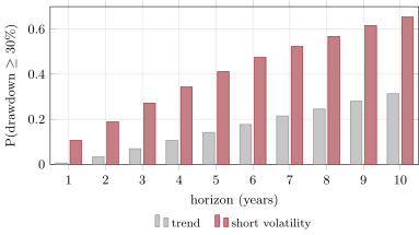
The probability of a drawdown of 30% or more within a horizon, over 4 000 simulated paths of each strategy’s model (long-run volatilities of 15% and 17%). Data: rs_perf.dd_probability. — **Figure 22.2.** The probability of a drawdown of 30% or more within a horizon, over 4 000 simulated paths of each strategy’s model (long-run volatilities of 15% and 17%). Data: `rs_perf.dd_probability`.

22.3 Turnover, hit rate and holding period

Definition 22.5 (Hit rate, profit factor)

The hit rate of a return stream is the share of its non-zero periods with a positive return. Its profit factor is the sum of its gains over the sum of its losses.

A hit rate says how often, not how much: the short-volatility stream wins on 76% of days and the trend stream on 53%, and the second has the better tail. A profit factor above one is a positive mean and nothing more; it equals the Omega ratio at zero (next section), since both are the mean gain over the mean loss. The market maker’s 65% of winning days and profit factor of 2.07 are those of a business collecting a spread with rare adverse days; its Sharpe ratio of 4.04 (standard error 0.45, HAC 0.52) is real and says nothing about capacity (chapter 28).

Turnover (chapter 16) sets costs, and with the gross exposure it sets the average holding period: a book of gross exposure $G$ that trades $T$ of capital one way per period replaces itself every $G/T$ periods. Chapter 16’s momentum book, rebuilt monthly on the 500 most liquid names, trades 1.86% of capital a day and holds a position for 48 trading days on average; its Sharpe ratio after costs is 0.17 with a standard error of 0.32 over ten years, and its longest drawdown lasted 2 079 of its 2 520 days. A strategy’s holding period should match its signal’s half-life (chapter 13); a holding period much shorter than the half-life is turnover paid for noise.

22.4 The shape of outcomes

Definition 22.6 (Sortino ratio, Omega ratio)

The Sortino ratio is the mean return in excess of a minimum acceptable return, divided by the downside deviation, the root mean square of the shortfalls below it (Sortino and Price). The Omega ratio at a threshold $L$ is $\mathbb{E}[(r-L)^+]\,/\,\mathbb{E}[(L-r)^+]$ , the expected gain above the threshold over the expected loss below it (Keating and Shadwick); it equals one at the mean.

Downside measures were designed to stop penalising strategies for their upside. They cannot see a downside the sample does not contain. In the displayed history the short-volatility stream’s daily returns have a skewness of $+5.38$ and a kurtosis of 102.5; over 100 simulated years the skewness is $-1.23$ and the kurtosis 121. The five years held rebounds, not crashes, and its Sortino ratio (1.87) and Omega ratio (1.49) beat the trend stream’s (1.48 and 1.17). Selling options raises the Sharpe ratio and the downside ratios of a history that has not yet met the options’ payoff; Goetzmann, Ingersoll, Spiegel and Welch showed how any of the popular measures can be gamed this way, and characterised a measure that cannot be: an average of a power utility over the return history.

The remedy is to measure the strategy, not the history: to know what the strategy is short of, to simulate or stress it where the history is silent (Book 6’s stress tests), and to read shape statistics as descriptions of a sample.

22.5 Benchmark-relative measures

Definition 22.7 (Market beta)

A strategy’s market beta is the slope of its returns on the market’s, $\beta = \operatorname{Cov}(r, r_m)/\operatorname{Var}(r_m)$ , estimated by regression with an intercept, the alpha (Book 1, chapter 1); standard errors are HAC.

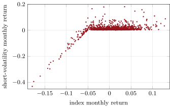
Regressed on the index it sells puts on, the short-volatility stream’s displayed history has a beta of 0.45 (standard error 0.09) and an annual alpha of 5.6% ( $t = 1.38$ ). A beta is a linear summary of a nonlinear exposure. Estimated separately on the index’s down days and up days, the history’s betas are 0.59 and 0.54; over 100 simulated years they are 0.98 and 0.71, and the monthly returns trace the payoff of a short put (Figure 22.3): flat above, steep below. The trend stream’s beta is 0.00 (0.03), with an alpha $t$ -statistic of 2.15 over five years; the market maker’s 0.04 (0.01), $t = 9.1$ . Against its benchmark a manager reports the information ratio and the tracking error (Book 1, chapter 3); the same caution applies.

Monthly returns of the short-volatility strategy against the index, over 100 simulated years: a short put’s payoff, with daily betas of 0.98 on down days and 0.71 on up days. Data: rs_perf.monthly_scatter. — **Figure 22.3.** Monthly returns of the short-volatility strategy against the index, over 100 simulated years: a short put’s payoff, with daily betas of 0.98 on down days and 0.71 on up days. Data: `rs_perf.monthly_scatter`.

22.6 Tutorial: four streams and a book

Goal. Compute firm.perf’s tear sheet for the four synthetic streams and chapter 16’s momentum book, and read what each number hides. End state: the tear-sheet table below, Figures 22.1, 22.2 and 22.3.

Lo’s annualisation: the per-period Sharpe ratio times $q/\sqrt{q + 2\sum(q-k)\rho_k}$ .

def lo_sharpe(r, q: int = 12, lags: int | None = None) -> float:
    """SR over q periods = q mu / sqrt(q gamma_0 + 2 sum_{k<q} (q - k) gamma_k): the per-period Sharpe ratio times
    q / sqrt(q + 2 sum (q - k) rho_k) instead of sqrt(q) (Lo 2002)."""
    x = returns_of(r)
    d = x - x.mean()
    n = len(x)
    L = q - 1 if lags is None else min(lags, q - 1)
    rho = [float(d[k:] @ d[:-k] / (d @ d)) for k in range(1, L + 1)]
    eta = q / math.sqrt(q + 2 * sum((q - k) * rho[k - 1] for k in range(1, L + 1)))
    return float(x.mean() / x.std(ddof=1) * eta) if n > 1 else float("nan")

Listing 22.1. The autocorrelation-adjusted Sharpe ratio. code/firm/perf/firm_perf.py

Drawdowns and their spells.

def drawdown(r, compound: bool = True) -> np.ndarray:
    w = np.r_[1.0, _wealth(returns_of(r), compound)]
    peak = np.maximum.accumulate(w)
    return (w / peak - 1)[1:] if compound else (w - peak)[1:]


def max_drawdown(r, compound: bool = True) -> float:
    return float(drawdown(r, compound).min())


def drawdown_spells(r, compound: bool = True):
    dd = drawdown(r, compound)
    spells, start = [], None
    for t, v in enumerate(dd):
        if v < 0 and start is None:
            start = t
        elif v >= 0 and start is not None:
            spells.append((start, start + int(np.argmin(dd[start:t])), t))
            start = None
    if start is not None:
        spells.append((start, start + int(np.argmin(dd[start:])), None))
    return spells


def longest_drawdown(r, compound: bool = True) -> int:
    n = len(returns_of(r))
    return max([(e if e is not None else n) - s for s, _, e in drawdown_spells(r, compound)], default=0)

Listing 22.2. Drawdown, maximum drawdown and drawdown spells. code/firm/perf/firm_perf.py

Unsmoothing: invert the moving average with the estimated profile.

def unsmooth(r, theta) -> np.ndarray:
    """r_t = (r_obs_t - sum_{j>=1} theta_j r_{t-j}) / theta_0, started from the observed mean (the start-up error
    decays geometrically when theta is invertible)."""
    x, th = returns_of(r), np.asarray(theta, float)
    out = np.full(len(x) + len(th) - 1, x.mean())
    k = len(th) - 1
    for t in range(len(x)):
        out[t + k] = (x[t] - th[1:] @ out[t + k - np.arange(1, k + 1)]) / th[0]
    return out[k:]

Listing 22.3. Recovering true returns from smoothed ones. code/firm/perf/firm_perf.py

Run rs_perf.histories(), stream_results(), momentum() and tear_sheet on each, then smoothed_report(), dd_probability() and fig_perf.py. The tear sheets, for five years of daily returns (the smoothed book: 60 months) and the momentum book’s ten years, with betas against the short-volatility simulation’s index and, for momentum, the synthetic market:

	trend	short vol.	smoothed	market maker	momentum
annual return	14.4%	11.6%	7.2%	22.8%	1.1%
annual volatility	14.6%	10.6%	7.4%	5.1%	9.1%
Sharpe ratio	1.00	1.09	0.99	4.04	0.17
standard error, iid	0.45	0.45	0.46	0.45	0.32
standard error, HAC	0.46	0.45	0.63	0.52	0.31
maximum drawdown	$-33.6$ %	$-14.8$ %	$-11.0$ %	$-4.2$ %	$-34.0$ %
longest drawdown	791 d	48 d	22 m	72 d	2 079 d
Calmar	0.43	0.78	0.66	5.39	0.03
Sortino	1.48	1.87	2.00	6.31	0.24
Omega at zero (profit factor)	1.17	1.49	2.07	2.07	1.03
skewness	$-0.04$	5.38	0.41	$-0.66$	0.00
kurtosis	3.0	102.5	2.8	9.9	3.4
hit rate	53%	76%	58%	65%	51%
market beta (HAC s.e.)	0.00 (0.03)	0.45 (0.09)		0.04 (0.01)	0.00 (0.01)

What to change next. Double the short-volatility notional and compare the displayed Sharpe ratio with the probability of a 30% drawdown; smooth the trend stream with the profile $(0.5, 0.3, 0.2)$ and see its Sharpe ratio rise by about 62%.

22.7 Build: the performance module

Purpose. One function reads any BacktestResult (or return stream) and reports the numbers of this chapter with their uncertainty, so that no strategy is judged on its Sharpe ratio alone.

Interface. from_returns(r, periods), sharpe, lo_sharpe(r, q, lags), drawdown, max_drawdown, drawdown_spells, longest_drawdown, calmar, sortino(r, periods, mar), omega(r, threshold), hit_rate, profit_factor, holding_period(res), alpha_beta(r, bench, periods, lags), smoothing_profile(r, k), unsmooth(r, theta), tear_sheet(res, bench, name, periods).

Rules. Every Sharpe ratio is printed with its standard error, iid and HAC; monthly or smoothed returns are annualised with their autocorrelations; drawdown probabilities come from a model of the strategy, not from its history’s maximum; shape statistics are labelled as the sample’s.

Acceptance tests. code/firm/perf/tests/: drawdowns, spells, Calmar, Sortino, Omega, hit rate and profit factor by hand; Lo’s ratio equal to $\sqrt q\,\mathrm{SR}_1$ on independent returns and correcting a smoothed stream; the smoothing profile recovered within 0.05 and the true returns recovered exactly after the start-up; a known beta and alpha; a holding period from known turnover.

Stretch. Deflated Sharpe ratios from the research log’s trial count (chapter 20); rolling tear sheets; the manipulation-proof measure.

Sources and further reading

A. W. Lo, “The statistics of Sharpe ratios”, Financial Analysts Journal 58(4), 2002.
M. Getmansky, A. W. Lo and I. Makarov, “An econometric model of serial correlation and illiquidity in hedge fund returns”, Journal of Financial Economics 74(3), 2004.
M. Magdon-Ismail, A. F. Atiya, A. Pratap and Y. S. Abu-Mostafa, “On the maximum drawdown of a Brownian motion”, Journal of Applied Probability 41(1), 2004.
F. Sortino and L. Price, “Performance measurement in a downside risk framework”, Journal of Investing 3(3), 1994; PerformanceAnalytics (R), documentation of SortinoRatio, CalmarRatio and Omega.
W. F. Sharpe, “Mutual fund performance”, Journal of Business 39(S1), 1966; “The Sharpe ratio”, Journal of Portfolio Management 21(1), 1994.
W. Goetzmann, J. Ingersoll, M. Spiegel and I. Welch, “Portfolio performance manipulation and manipulation-proof performance measures”, Review of Financial Studies 20(5), 2007.

22.8 Exercises

Exercise 22.1 ★

A strategy has a Sharpe ratio of 1.0 over five years of daily returns. What is its standard error, and its 95% interval?

Solution

Solution of Exercise 22.1.

About $\sqrt{252/1\,260} = 0.45$ (the $\mathrm{SR}^2/2$ term is negligible per day); the 95% interval runs from 0.12 to 1.88.

Exercise 22.2 ★

The trend stream returned 14.4% a year with a maximum drawdown of 33.6%. Compute its Calmar ratio. Why is the Calmar ratio of a single history unstable?

Solution

Solution of Exercise 22.2.

$0.144/0.336 = 0.43$ . The maximum drawdown is one draw from a wide distribution: the same strategy’s five-year maximum exceeds 30% in 14% of paths and stays far below it in most; a ratio with one extreme in its denominator inherits that instability.

Exercise 22.3 ★

Show that the profit factor equals the Omega ratio at a threshold of zero.

Solution

Solution of Exercise 22.3.

Over $n$ periods, $\sum r^+ / \sum r^- = (\frac1n\sum r^+)/(\frac1n\sum r^-) = \mathbb{E}_n[(r - 0)^+]/\mathbb{E}_n[(0 - r)^+]$ , the sample Omega ratio at zero.

Exercise 22.4 ★★

True returns with a Sharpe ratio of 0.6 are reported smoothed with the profile $(0.5, 0.3, 0.2)$ . Give the factor on the variance, on the volatility, the reported Sharpe ratio, and the first two autocorrelations.

Solution

Solution of Exercise 22.4.

$\sum\theta_j^2 = 0.25 + 0.09 + 0.04 = 0.38$ ; volatility factor $\sqrt{0.38} = 0.616$ ; reported Sharpe ratio $0.6/0.616 = 0.97$ ; $\rho_1 = (0.5 \times 0.3 + 0.3 \times 0.2)/0.38 = 0.55$ , $\rho_2 = 0.5 \times 0.2/0.38 = 0.26$ .

Exercise 22.5 ★★

With the autocorrelations of exercise 4 (and zero beyond lag 2), compute Lo’s annualisation factor for monthly returns and compare it with $\sqrt{12}$ . By how much does the naive annualisation overstate the Sharpe ratio?

Solution

Solution of Exercise 22.5.

$12/\sqrt{12 + 2(11 \times 0.55 + 10 \times 0.26)} = 2.22$ against $\sqrt{12} = 3.46$ : the naive annualisation overstates the Sharpe ratio by a factor of $3.46/2.22 = 1.56$ , 56%.

Exercise 22.6 ★★

Why does a beta of 0.45 understate the short-volatility strategy’s exposure to a crash? Use the down- and up-day betas.

Solution

Solution of Exercise 22.6.

The beta averages a kinked payoff: over 100 simulated years the daily beta is 0.98 on the index’s down days and 0.71 on up days, and in a crash the put’s delta rises towards one, so the loss is far larger than 0.45 times the index’s fall. The displayed history (0.59 and 0.54) holds no crash to reveal the kink.

Exercise 22.7 ★★★

Coding. With rs_perf.dd_probability, give the probability of a 30% drawdown within one year and within ten for each strategy, and explain why the short-volatility strategy’s probability starts so much higher.

Solution

Solution of Exercise 22.7.

Within one year: 0.6% for the trend strategy, 11% for short volatility; within ten years: 31% and 65%. The short-volatility strategy’s losses come in jumps (a crash month takes a large share of capital at once), so a 30% fall does not need the slow accumulation of bad days a diffusion needs.

Exercise 22.8 ★★★

Find the flaw. “Our fund’s Sortino ratio is 1.9 and it has never had a losing quarter in five years, so its downside risk is lower than that of the trend fund next door, whose Sortino ratio is 1.5 and which lost a third of its value.”

Solution

Solution of Exercise 22.8.

The fund’s Sortino ratio (1.87 in the chapter’s example) and its record come from a history without a crash; a downside measure cannot see a downside the sample lacks. Its model gives a 41% chance of a 30% drawdown in five years against the trend fund’s 14%, and over 100 years its skewness is $-1.23$ . Measure the strategy’s exposure (a short put) and stress it, not the history.

22.9 Problem: Two Sharpe Ratios of One

Problem 22.1

Weekend problem — two Sharpe ratios of one

The chapter’s four streams and chapter 16’s momentum book, through firm.perf.

Part I — The Sharpe ratio.

What are the Sharpe ratios of the trend and short-volatility histories, and their standard errors?
Why do four of the five streams have nearly the same standard error?
What does the HAC standard error say about the smoothed book?
What is the market maker’s Sharpe ratio and its standard error, and what does it not tell you?

Part II — Smoothing.

What are the smoothed book’s reported and true volatilities?
What are its reported, Lo-adjusted, unsmoothed and true Sharpe ratios?
Which smoothing profile is estimated, from which autocorrelations?
Why is the naive annualisation wrong for this book?

Part III — Drawdowns and shape.

Give each displayed history’s maximum drawdown and longest drawdown.
Which strategy has the better Calmar, Sortino and Omega ratios in the displayed histories, and which has the worse tail?
What are the short-volatility stream’s skewness and kurtosis in the history and over 100 years?
What share of its five-year histories have no losing quarter?
What are the momentum book’s holding period and turnover?

Part IV — The verdict.

State the named result: the probability of a 30% drawdown within five years for each strategy, and the Sharpe ratio’s standard error under the smoothed book’s autocorrelation.
What do 200 simulated years give for each strategy’s Sharpe ratio and maximum drawdown?
What are the short-volatility strategy’s beta, down-day and up-day betas?
Which of the two would you allocate to, and how would you size it?
What should every tear sheet print next to a Sharpe ratio?
How could a manager game the measures of this chapter?
In one sentence: what does a Sharpe ratio of one over five years tell you?

Solution

Solution of Problem 22.1.

1.00 and 1.09, each with an iid standard error of 0.45 (HAC 0.46 and 0.45).
The standard error depends on the length of the history in years, about $\sqrt{q/T}$ , and all four span five years.
0.63 against 0.46: serially correlated returns carry less information than their number suggests.
4.04 with a standard error of 0.45 (HAC 0.52): a real edge, but nothing about capacity, crowding or what an adverse day can cost at size.
7.4% reported, 11.2% true.
0.99 reported, 0.61 with Lo’s correction, 0.59 unsmoothed, 0.66 true.
$(0.43, 0.36, 0.21)$ , from first autocorrelations of 0.64 and 0.25.
Its returns are autocorrelated, so the volatility of a year’s sum is larger than $\sqrt{12}$ times the monthly volatility.
Trend $-33.6\%$ and 791 days; short volatility $-14.8\%$ and 48 days; smoothed $-11.0\%$ and 22 months; market maker $-4.2\%$ and 72 days.
The short-volatility history on all three (Calmar 0.78, Sortino 1.87, Omega 1.49 against 0.43, 1.48, 1.17); it also has the worse tail.
$+5.38$ and 102.5 in the history; $-1.23$ and 121 over 100 years.
9%.
48 trading days; a one-way turnover of 1.86% of capital a day.
Named result. A 30% drawdown within five years: 14% for the trend strategy, 41% for short volatility. The smoothed book’s Sharpe ratio has a standard error of 0.63 with its autocorrelation (HAC) against 0.46 assuming independence.
Trend: 0.83 and $-37\%$ . Short volatility: 0.62 and $-72\%$ .
0.45 (standard error 0.09) in the history; down-day and up-day betas of 0.59 and 0.54 in the history, 0.98 and 0.71 over 100 years.
The trend strategy, or the short-volatility one only sized to its crash (a stress loss within the drawdown budget), not to its history’s volatility.
Its standard error (iid and HAC), the length of the history, the number of trials behind it, and the drawdown probability of the strategy’s model.
Sell options or other tail risk, smooth marks, or choose the reporting window; a manipulation-proof measure or a stress test answers each.
That the strategy’s true Sharpe ratio is probably between 0.1 and 1.9, and nothing about its tail.

22.10 Interview questions

Interview question 22.1 ★ researcher, trader

A strategy shows a Sharpe ratio of 1 over three years of daily data. How confident are you that it is positive?

Solution

Solution of Interview question 22.1.

The standard error is about $\sqrt{252/756} = 0.58$ , so the estimate is 1.7 standard errors from zero: fairly but not very confident, before any correction for the number of strategies tried (chapter 20).

Interview question 22.2 ★★ researcher, risk

How can a strategy raise its Sharpe ratio without adding skill? How would you detect it?

Solution

Solution of Interview question 22.2.

Sell out-of-the-money options or other tail risk (steady gains, rare large losses), smooth the marks of illiquid positions, or pick the window. Look at the shape across a long simulated or stressed history, the down-market beta, the autocorrelation of returns, and the positions themselves; Goetzmann and co-authors give a measure that cannot be gamed.

Interview question 22.3 ★★ researcher

A fund’s monthly returns have a first autocorrelation of 0.6. What does that do to its Sharpe ratio, and how do you correct it?

Solution

Solution of Interview question 22.3.

It inflates the annualised Sharpe ratio (stale marks lower the measured volatility) and makes it less precise. Correct with Lo’s autocorrelation-adjusted annualisation, unsmooth the returns with the estimated profile of Getmansky, Lo and Makarov, and use HAC standard errors.

Interview question 22.4 ★★ risk

How does the expected maximum drawdown of a strategy grow with the horizon? Why is a backtest’s maximum drawdown a poor risk estimate?

Solution

Solution of Interview question 22.4.

For a Brownian motion with positive drift it grows logarithmically with the horizon (square root with no drift). A backtest’s maximum is a single draw, and it cannot contain the events the sample lacks; use the distribution of drawdowns under a model and stress tests.

Interview question 22.5 ★★ trader

A market maker wins on 65% of days with a Sharpe ratio of 4. What would you still want to know?

Solution

Solution of Interview question 22.5.

The loss distribution of its bad days (the 1.5% adverse-selection days), capacity and how the edge scales with size, its inventory limits, the correlation of its losses with market stress, and whether the P&L decomposes into spread capture and adverse selection that make sense (chapter 23).

Interview question 22.6 ★★★ researcher

Derive the standard error of the Sharpe ratio for independent normal returns.

Solution

Solution of Interview question 22.6.

With $\hat\mu$ and $\hat\sigma^2$ independent for normal data, $\operatorname{Var}\hat\mu = \sigma^2/T$ and $\operatorname{Var}\hat\sigma^2 = 2\sigma^4/T$ . The delta method on $\mathrm{SR} = \mu/\sigma$ , with derivatives $1/\sigma$ and $-\mu/(2\sigma^3)$ , gives $\operatorname{Var}\widehat{\mathrm{SR}} = 1/T + \mu^2/(2\sigma^2 T) = (1 + \mathrm{SR}^2/2)/T$ .

Terms defined in this chapter

See all 2333 terms in the glossary