University Mathematics — Year 1 · Bachelor Year 1

5Linear Differential Equations

First met in the High School volume, differential equations are treated here with full proofs and in greater generality: first-order linear equations with variable coefficients (solved completely by the variation-of-constants method) and second-order linear equations with constant coefficients, the model for oscillations. Both cases display the same structure: general solution $=$ one particular solution $+$ general solution of the homogeneous equation.

5.1 First-order linear equations

Definition 5.1

Let $I$ be an interval and $a, b \colon I \to \R$ (or $\C$ ) be continuous. The equation

(E)\colon\quad y' + a(x)\,y = b(x),

in the unknown differentiable function $y \colon I \to \R$ (or $\C$ ), is a first-order linear differential equation. The equation $(H)\colon y' + a(x) y = 0$ is its homogeneous equation.

Theorem 5.2 (Solving the homogeneous equation)

Let $A$ be a primitive of $a$ on $I$ (it exists: Chapter 15). The solutions of $(H)$ on $I$ are exactly the functions

y(x) = \lambda\, \eu^{-A(x)}, \qquad \lambda \in \R \text{ (or } \C).

Proof. These functions are solutions: $y' = -\lambda A' \eu^{-A} = -a y$ . Conversely, let $y$ solve $(H)$ and set $z(x) = y(x)\, \eu^{A(x)}$ . Then

z' = y' \eu^{A} + y\, a\, \eu^{A} = (y' + ay)\, \eu^{A} = 0 ,

so $z$ is constant on the interval $I$ , say $z = \lambda$ : $y = \lambda \eu^{-A}$ . (Note the logic: no solution is lost, because every solution has been written in the announced form.) ∎

Example 5.3 (A homogeneous equation with variable coefficient)

Solve $y' + (\cos x)\,y = 0$ on $\R$ . A primitive of $a(x) = \cos x$ is $A(x) = \sin x$ , so the solutions are

y(x) = \lambda\,\eu^{-\sin x}, \qquad \lambda \in \R .

Two readings. Every solution is periodic (period $2\pi$ ) and never vanishes unless $\lambda = 0$ — the sign of $\lambda$ is the sign of $y$ forever, since an exponential cannot cross zero. And the solution through $y(0) = y_0$ is $y_0\eu^{-\sin x}$ : exactly one curve of the family through each initial point, the one-dimensional picture of Theorem 5.4 (2).

Theorem 5.4 (Variation of constants; Cauchy problem)

With the notation above:

The solutions of $(E)$ on $I$ are exactly

$y(x) = \Bigl(\lambda + \int_{x_0}^{x} b(t)\, \eu^{A(t)} \dd t \Bigr)\, \eu^{-A(x)}, \qquad \lambda \in \R,$

where $x_0 \in I$ is fixed. Equivalently: general solution of $(H)$ plus one particular solution of $(E)$ .
For every $x_0 \in I$ and $y_0$ , the Cauchy problem “ $(E)$ and $y(x_0) = y_0$ ” has exactly one solution on $I$ .

Proof. (1) Following the method named variation of constants, look for solutions of the form $y = \mu(x)\, \eu^{-A(x)}$ with $\mu$ differentiable — no generality is lost, since every function on $I$ can be so written ( $\mu = y\,\eu^{A}$ ). Substituting,

y' + ay = \mu' \eu^{-A} - \mu a \eu^{-A} + a\mu\eu^{-A} = \mu'\, \eu^{-A},

so $y$ solves $(E)$ if and only if $\mu'(x) = b(x)\,\eu^{A(x)}$ , if and only if $\mu(x) = \lambda + \int_{x_0}^x b(t)\eu^{A(t)}\dd t$ for some constant $\lambda$ (two primitives of the same continuous function on an interval differ by a constant).

(2) In the formula, $y(x_0) = \lambda\,\eu^{-A(x_0)}$ : the condition $y(x_0) = y_0$ determines $\lambda = y_0 \eu^{A(x_0)}$ uniquely. ∎

Example 5.5

Solve $y' + \dfrac{y}{x} = x^2$ on $I = \intoo{0}{+\infty}$ . Here $a(x) = \frac 1x$ , $A(x) = \ln x$ , $\eu^{-A(x)} = \frac 1x$ . Homogeneous solutions: $\frac{\lambda}{x}$ . Variation of constants: $\mu'(x) = x^2 \cdot x = x^3$ , so $\mu = \frac{x^4}{4} + \lambda$ , and

y(x) = \frac{x^3}{4} + \frac{\lambda}{x}, \qquad \lambda \in \R .

With the initial condition $y(1) = 0$ : $\lambda = -\frac14$ . Check: $y' + \frac yx = \frac{3x^2}{4} - \frac{\lambda}{x^2} + \frac{x^2}{4} + \frac{\lambda}{x^2} = x^2$ .

Example 5.6 (Guessing beats integrating)

Solve $y' + 2x\,y = x$ on $\R$ . Variation of constants works ( $A = x^2$ , $\mu' = x\,\eu^{x^2}$ , $\mu = \frac12\eu^{x^2} + \lambda$ ), but observing that the constant $y_p = \frac12$ solves the equation ( $0 + 2x\cdot\frac12 = x$ ) is faster. With the homogeneous solutions $\lambda\,\eu^{-x^2}$ :

y(x) = \frac12 + \lambda\,\eu^{-x^2}, \qquad \lambda \in \R .

Every solution converges to $\frac12$ extremely fast as $x \to \pm\infty$ : the constant particular solution is an equilibrium that all solutions join. The insight: before launching the general method, spend ten seconds looking for an obvious particular solution (constant, monomial, multiple of the right-hand side); the structure theorem then finishes the job.

Remark 5.7 (Intervals matter)

The theorem lives on an interval where $a$ and $b$ are continuous. For $y' + \frac yx = 0$ on $\R^*$ , the solutions are $\frac{\lambda}{x}$ on $\intoo{0}{+\infty}$ and $\frac{\mu}{x}$ on $\intoo{-\infty}{0}$ with independent constants: there is no reason for a single formula to glue across the singularity at $0$ .

Example 5.8 (A complex right-hand side, two real answers)

Solve $y' - y = \cos x$ and $y' - y = \sin x$ in one stroke. Work in $\C$ with the right-hand side $\eu^{\iu x}$ : trying $y_p = c\,\eu^{\iu x}$ gives $c(\iu - 1)\eu^{\iu x} = \eu^{\iu x}$ , so

c = \frac1{\iu - 1} = \frac{-1 - \iu}2, \qquad y_p = -\frac{(1 + \iu)(\cos x + \iu\sin x)}2 = \frac{\sin x - \cos x}2 + \iu\,\frac{-\sin x - \cos x}2 .

Since the equation has real coefficients, real and imaginary parts split: $\frac{\sin x - \cos x}2$ solves $y' - y = \cos x$ , and $-\frac{\sin x + \cos x}2$ solves $y' - y = \sin x$ (check the first: derivative $\frac{\cos x + \sin x}2$ , minus the function, gives $\cos x$ ). One complex line replaced two runs of variation of constants — the same economy that Method 5.13 systematizes for second order, and a recurring dividend of Chapter 3.

5.2 Second-order linear equations with constant coefficients

Definition 5.9

Let $a, b \in \R$ and $f \colon I \to \R$ continuous. The equation

(E)\colon\quad y'' + a\,y' + b\,y = f(x)

is a second-order linear equation with constant coefficients; $(H)\colon y'' + ay' + by = 0$ is its homogeneous equation, and $\chi(r) = r^2 + ar + b$ its characteristic polynomial.

Theorem 5.10 (Homogeneous solutions)

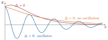
Let $\Delta = a^2 - 4b$ be the discriminant of $\chi$ . The real solutions of $(H)$ on $\R$ are:

if $\Delta > 0$ , with $r_1 \neq r_2$ the two real roots: $\;y = \lambda\, \eu^{r_1 x} + \mu\, \eu^{r_2 x}$ ;
if $\Delta = 0$ , with $r_0$ the double root: $\;y = (\lambda + \mu x)\, \eu^{r_0 x}$ ;
if $\Delta < 0$ , with roots $\alpha \pm \iu\omega$ ( $\omega > 0$ ): $\;y = \eu^{\alpha x} (\lambda \cos\omega x + \mu \sin\omega x)$ ;

in each case with $(\lambda, \mu)$ running over $\R^2$ .

Proof. First observe that for $r \in \C$ , $x \mapsto \eu^{rx}$ solves $(H)$ if and only if $\chi(r) = 0$ (substitute: $(r^2 + ar + b)\eu^{rx} = 0$ ). This is why exponentials are the natural first guess: differentiation acts on $\eu^{rx}$ as multiplication by the number $r$ , so the differential equation becomes the numerical equation $\chi(r) = 0$ — the whole analytic problem is compressed into finding the roots of one quadratic.

The key step is a change of unknown that reduces the order. Let $r$ be a (possibly complex) root of $\chi$ and write $y = z\, \eu^{rx}$ , which loses no generality. Then

y'' + ay' + by = \bigl(z'' + (2r + a) z' + \chi(r) z\bigr)\eu^{rx} = \bigl(z'' + (2r + a) z'\bigr)\eu^{rx},

so $(H)$ becomes the first-order equation $u' + (2r + a) u = 0$ for $u = z'$ .

Case $\Delta \neq 0$ : choose $r = r_1$ ; then $2r_1 + a = r_1 - r_2$ (since $r_1 + r_2 = -a$ ). By Theorem 5.2, $z' = c\,\eu^{(r_2 - r_1)x}$ for some constant $c$ ; integrating on $\R$ , $z = \mu\, \eu^{(r_2 - r_1)x} + \lambda$ with $\mu = \frac{c}{r_2 - r_1}$ , and therefore $y = z\, \eu^{r_1 x} = \lambda\,\eu^{r_1x} + \mu\,\eu^{r_2x}$ . When $\Delta < 0$ , the roots are $\alpha \pm \iu\omega$ and the complex solutions are $y = c_1\eu^{(\alpha+\iu\omega)x} + c_2\eu^{(\alpha-\iu\omega)x}$ with $c_1, c_2 \in \C$ . Which of these are real-valued? Since $\conj{\eu^{(\alpha+\iu\omega)x}} = \eu^{(\alpha-\iu\omega)x}$ , the conjugate of $y$ is $\conj{c_2}\, \eu^{(\alpha+\iu\omega)x} + \conj{c_1}\,\eu^{(\alpha-\iu\omega)x}$ , and $y = \conj y$ for all $x$ forces $c_2 = \conj{c_1}$ (the two exponentials are linearly independent: evaluate at two points, or compare at $x=0$ after dividing by $\eu^{\alpha x}$ ). Writing $c_1 = \frac{\lambda - \iu\mu}2$ with $\lambda, \mu$ real:

y = 2\,\Re\Bigl(c_1\,\eu^{\alpha x}(\cos\omega x + \iu\sin\omega x)\Bigr) = \eu^{\alpha x}\bigl(\lambda\cos\omega x + \mu\sin\omega x\bigr),

and conversely every such function is a solution (real part of a complex solution of a real equation): the real solution space is as announced.

Case $\Delta = 0$ : $r = r_0$ , $2r_0 + a = 0$ , so $z'' = 0$ : $z = \lambda + \mu x$ and $y = (\lambda + \mu x)\eu^{r_0 x}$ . ∎

Example 5.11 (A Cauchy problem, start to finish)

Solve $y'' - 3y' + 2y = 0$ with $y(0) = 0$ , $y'(0) = 1$ . The characteristic polynomial $r^2 - 3r + 2 = (r - 1)(r - 2)$ has the real roots $1$ and $2$ : general solution $y = \lambda\eu^{x} + \mu\eu^{2x}$ . The two conditions give the linear system

\lambda + \mu = 0, \qquad \lambda + 2\mu = 1 ,

so $\mu = 1$ , $\lambda = -1$ :

y(x) = \eu^{2x} - \eu^{x} .

Check: $y(0) = 0$ ; $y' = 2\eu^{2x} - \eu^x$ has $y'(0) = 1$ ; and $y'' - 3y' + 2y = (4 - 6 + 2)\eu^{2x} + (-1 + 3 - 2)\eu^x = 0$ . Note the shape of the answer: near $-\infty$ the slow mode $-\eu^x$ dominates; near $+\infty$ the fast mode $\eu^{2x}$ does. Reading solutions as superpositions of modes with different decay or growth rates is the profitable habit — it is how the transient/steady-state split of the weekend problem is organized.

The three regimes of y'' + ay' + by = 0 with decaying solutions: damped oscillation (complex roots), critical return (double root), overdamped decay (two real roots). Which regime occurs is read off the sign of = a2 - 4b alone — before solving anything. — The three regimes of $y'' + ay' + by = 0$ with decaying solutions: damped oscillation (complex roots), critical return (double root), overdamped decay (two real roots). Which regime occurs is read off the sign of $\Delta = a^2 - 4b$ alone — before solving anything.

Theorem 5.12 (Structure and Cauchy problem)

If $y_p$ is one particular solution of $(E)$ , the solutions of $(E)$ are exactly $y_p + y_h$ , $y_h$ running over the solutions of $(H)$ .
(Superposition) If $y_1$ solves $y'' + ay' + by = f_1$ and $y_2$ solves $y'' + ay' + by = f_2$ , then $y_1 + y_2$ solves the equation with right-hand side $f_1 + f_2$ .
For all $x_0 \in I$ and $(y_0, y_0')$ , the Cauchy problem “ $(E)$ , $y(x_0) = y_0$ , $y'(x_0) = y_0'$ ” has exactly one solution on $I$ . (Existence granted a particular solution; uniqueness in full.)

Proof. (1) $y$ solves $(E)$ iff $y - y_p$ solves $(H)$ , by linearity of $y \mapsto y'' + ay' + by$ . (2) is the same linearity.

(3) By (1) it suffices to prove that the constants $(\lambda, \mu)$ can always be adjusted, uniquely, to any data $(y_0, y_0')$ . Translating the variable, assume $x_0 = 0$ . In case (1) of Theorem 5.10, $y = \lambda\eu^{r_1x} + \mu\eu^{r_2x}$ gives

y(0) = \lambda + \mu, \qquad y'(0) = r_1\lambda + r_2\mu :

a linear system in $(\lambda, \mu)$ whose determinant is $r_2 - r_1 \neq 0$ ; solving it explicitly, $\mu = \frac{y_0' - r_1y_0}{r_2 - r_1}$ and $\lambda = y_0 - \mu$ : exactly one solution. In case (2), $y(0) = \lambda$ and $y'(0) = r_0\lambda + \mu$ : the system is triangular with determinant $1$ , solved by $\lambda = y_0$ , $\mu = y_0' - r_0y_0$ . In case (3), $y(0) = \lambda$ and $y'(0) = \alpha\lambda + \omega\mu$ : determinant $\omega \neq 0$ , solved by $\lambda = y_0$ , $\mu = \frac{y_0' - \alpha y_0}\omega$ . In each case the map $(\lambda, \mu) \mapsto (y(x_0), y'(x_0))$ is a linear bijection — the language of Chapter 20 will compress this case check into one sentence. ∎

Method 5.13 (Particular solution for $f(x) = P(x)\,\eu^{\gamma x}$ )

When the right-hand side is $P(x)\,\eu^{\gamma x}$ with $P$ a polynomial and $\gamma \in \R$ (this covers polynomials, exponentials, and via complex $\gamma$ or superposition, $\cos$ and $\sin$ ): look for a particular solution of the form

y_p(x) = x^{m}\, Q(x)\, \eu^{\gamma x}, \qquad m = \text{multiplicity of } \gamma \text{ as a root of } \chi \ (m = 0, 1 \text{ or } 2),

with $Q$ a polynomial of the same degree as $P$ , whose coefficients are found by substitution and identification. For $f = K\cos\omega x$ (or $\sin$ ), solve with right-hand side $K\eu^{\iu\omega x}$ and take the real (resp. imaginary) part.

Example 5.14 (Superposition in action)

Solve $y'' - y = \eu^{x} + 4$ on $\R$ . Homogeneous: $\chi(r) = r^2 - 1$ , roots $\pm1$ , so $y_h = \lambda\eu^x + \mu\eu^{-x}$ . Split the right-hand side and treat each piece by the method box. Piece $\eu^x$ : here $\gamma = 1$ is a simple root of $\chi$ , so try $y_1 = c\,x\,\eu^x$ : then $y_1'' - y_1 = c(x + 2)\eu^x - cx\eu^x = 2c\,\eu^x$ , giving $c = \frac12$ . Piece $4$ : $\gamma = 0$ is not a root; the constant $y_2 = -4$ works. By superposition (Theorem 5.12 (2)):

y = \frac{x\,\eu^x}2 - 4 + \lambda\,\eu^x + \mu\,\eu^{-x}, \qquad (\lambda, \mu) \in \R^2 .

Note how the two pieces demanded different shapes ( $m = 1$ versus $m = 0$ ): the multiplicity test is applied to each exponent separately, which is the whole point of splitting the right-hand side before guessing.

Example 5.15 (The multiplicity rule at work)

Solve $y'' + y' = x$ on $\R$ . The right-hand side is $P(x)\eu^{0 \cdot x}$ with $P(x) = x$ , and $\gamma = 0$ is a simple root of $\chi(r) = r^2 + r = r(r + 1)$ : so $m = 1$ , and the correct guess is $y_p = x\,(\alpha x + \beta) = \alpha x^2 + \beta x$ , one degree higher than $P$ . Substituting:

y_p'' + y_p' = 2\alpha + (2\alpha x + \beta) = 2\alpha x + (2\alpha + \beta) ,

and identification with $x$ gives $\alpha = \frac12$ , $\beta = -1$ : $y_p = \frac{x^2}2 - x$ . General solution: $y = \frac{x^2}2 - x + \lambda + \mu\,\eu^{-x}$ . Had we guessed $y_p = \alpha x + \beta$ (ignoring the multiplicity), substitution would give $y_p'' + y_p' = \alpha$ , a constant — no choice of $\alpha, \beta$ can match $x$ , and the failure is structural: constants already solve the homogeneous equation, so they are invisible to the left-hand side. The factor $x^m$ exists precisely to climb out of the homogeneous solution space.

Remark 5.16 (The thirty-second insurance policy)

Every solved equation in this chapter ends with a substitution check, and this is not decorative. A differential-equation computation chains many small steps (a primitive, a product rule, two constants), and a single sign error propagates invisibly; substituting the final formula back into the equation catches essentially all of them at the cost of one differentiation. Cultivate the reflex in three layers: check the particular solution alone (the homogeneous part cancels anyway), check the initial conditions on the full solution, and when a parameter is present, check a degenerate value (does the formula for general $\Omega$ reproduce the known answer at $\Omega = 0$ ?). The habit costs half a minute; it converts “probably right” into “verified”.

Remark 5.17 (Common pitfalls)

Normalize first. The formulas assume the equation reads $y' + a(x)y = b(x)$ — coefficient $1$ on $y'$ . For $xy' - 2y = x^3$ , divide by $x$ (on an interval avoiding $0$ ) before identifying $a$ and $b$ , as in Exercise 5.2.
One constant per dimension, fixed at the end. The general first-order solution carries one constant, the second-order one two; initial conditions are imposed on the complete solution $y_p + y_h$ , never on $y_h$ alone — imposing them before adding $y_p$ is the most frequent structural error.
Mind the multiplicity. A particular-solution guess that solves the homogeneous equation is invisible to the left-hand side; the factor $x^m$ of Method 5.13 is not optional (Example 5.15).
Intervals are part of the answer. Solutions live on intervals where the coefficients are continuous; gluing across a singularity can create spurious constants (Exercise 5.12) or destroy uniqueness. “Solve on $\R^*$ ” means two independent problems.

Example 5.18 (Off-resonance forcing)

Solve $y'' + 4y = \sin x$ on $\R$ . Natural frequency $2$ , forcing frequency $1$ : since $\iu$ is not a root of $\chi(r) = r^2 + 4$ , the multiplicity is $m = 0$ and a plain sinusoid suffices. Trying $y_p = \alpha\sin x$ (no cosine needed: the equation has no $y'$ term, and $\sin$ regenerates $\sin$ ):

y_p'' + 4y_p = -\alpha\sin x + 4\alpha\sin x = 3\alpha\sin x ,

so $\alpha = \frac13$ and the general solution is

y = \frac{\sin x}3 + \lambda\cos 2x + \mu\sin 2x .

Every solution stays bounded: a superposition of two oscillations at the frequencies $1$ (forced) and $2$ (natural). Compare with the next example, where forcing at the natural frequency changes the answer’s very shape.

Example 5.19 (A forced oscillation)

Solve $y'' + y = \cos x$ , $y(0) = 0$ , $y'(0) = 0$ .

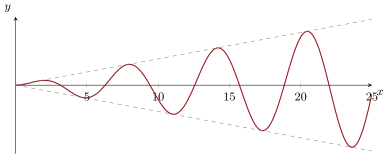
Homogeneous: $\chi(r) = r^2 + 1$ , roots $\pm\iu$ : $y_h = \lambda\cos x + \mu \sin x$ .

Particular: right-hand side $\Re(\eu^{\iu x})$ with $\gamma = \iu$ a simple root of $\chi$ : try $z_p = c\, x\, \eu^{\iu x}$ ( $c \in \C$ ). Then $z_p'' + z_p = c\,(2\iu)\eu^{\iu x}$ , which equals $\eu^{\iu x}$ for $c = \frac{1}{2\iu} = -\frac\iu2$ . So $z_p = -\frac{\iu}{2} x (\cos x + \iu \sin x)$ and $y_p = \Re(z_p) = \frac{x \sin x}{2}$ .

General solution: $y = \frac{x\sin x}{2} + \lambda\cos x + \mu\sin x$ . Conditions: $y(0) = \lambda = 0$ ; $y' = \frac{\sin x + x\cos x}{2} + \mu\cos x$ , so $y'(0) = \mu = 0$ . Answer: $y = \frac{x\sin x}{2}$ — an oscillation whose amplitude grows linearly: the resonance phenomenon, caused by forcing the system at its natural frequency.

Resonance: the solution y = x x/2 of y'' + y = x oscillates between the lines y = ± x2 (dashed), with ever-growing amplitude. — Resonance: the solution $y = \frac{x \sin x}{2}$ of $y'' + y = \cos x$ oscillates between the lines $y = \pm\frac x2$ (dashed), with ever-growing amplitude.

Remark 5.20 (Interlude: linearity is a geometry)

Look back at the shape of every solution set in this chapter: a special solution plus a space of homogeneous solutions with one free constant (first order) or two (second order). The chapters on linear algebra (Chapters 18, 19 and 20) will supply the exact vocabulary: the map $L(y) = y'' + ay' + by$ is linear, its homogeneous solutions form the kernel of $L$ , a vector space whose dimension equals the order of the equation — that is the honest content of “one constant per order” — and the solution set of $L(y) = f$ is an affine subspace, a translate of the kernel. Even the Cauchy map $(\lambda, \mu) \mapsto (y(x_0), y'(x_0))$ of Theorem 5.12 is a linear bijection between two planes, i.e. an invertible $2 \times 2$ system (Chapter 21). Nothing in this chapter will need to be redone — it will only need to be renamed, and the renaming is the best possible warm-up for linear algebra: every abstract definition there has already earned its living here.

Remark 5.21 (Where this chapter is used)

The structure theorem — solutions of $(E)$ form “a particular solution plus the solutions of $(H)$ ” — is the first appearance of a pattern that Chapters 18 and 20 will name: the solution set of $(H)$ is the kernel of the linear map $y \mapsto y'' + ay' + by$ , and the solution set of $(E)$ is an affine translate of it. The characteristic polynomial reappears as the characteristic polynomial of a matrix in Chapter 21: a second-order equation is a $2 \times 2$ first-order system in disguise, a viewpoint the Year 2 volume systematizes. The integrals demanded by variation of constants are supplied by Chapter 15, and the weekend problem below — the driven damped oscillator — is the model case for every oscillation question in the sciences, from circuits to suspension bridges.

5.3 Exercises

Exercise 5.1 ★

Solve on $\R$ : $\;y' + 2y = \eu^{3x}$ ; then the Cauchy problem $y(0) = 1$ .

Solution

Solution of Exercise 5.1.

Homogeneous: $y_h = \lambda\,\eu^{-2x}$ . Particular: try $y_p = c\,\eu^{3x}$ ( $3$ is not a root of $r + 2$ ): $3c + 2c = 1$ , $c = \frac15$ . General solution: $y = \frac{\eu^{3x}}{5} + \lambda\,\eu^{-2x}$ . With $y(0) = 1$ : $\frac15 + \lambda = 1$ , $\lambda = \frac45$ , so $y = \frac{\eu^{3x} + 4\,\eu^{-2x}}{5}$ .

Exercise 5.2 ★

Solve on $\intoo{0}{+\infty}$ : $\;x y' - 2y = x^3$ (put the equation in the normalized form first).

Solution

Solution of Exercise 5.2.

On $\intoo{0}{+\infty}$ , divide by $x$ : $y' - \frac{2}{x}\,y = x^2$ . Here $A(x) = -2\ln x$ , $\eu^{-A(x)} = x^2$ : homogeneous solutions $\lambda x^2$ . Variation of constants: $\mu'(x) = x^2 \cdot x^{-2} = 1$ , so $\mu = x + \lambda$ and

y(x) = x^3 + \lambda x^2, \qquad \lambda \in \R .

Check: $x(3x^2 + 2\lambda x) - 2(x^3 + \lambda x^2) = x^3$ .

Exercise 5.3 ★

Solve on $\R$ , giving the real general solution: $\;y'' - 3y' + 2y = 0$ ; $\;y'' + 4y' + 4y = 0$ ; $\;y'' - 2y' + 5y = 0$ .

Solution

Solution of Exercise 5.3.

$y'' - 3y' + 2y = 0$ : roots $1$ and $2$ ; $\;y = \lambda\,\eu^{x} + \mu\,\eu^{2x}$ .

$y'' + 4y' + 4y = 0$ : double root $-2$ ; $\;y = (\lambda + \mu x)\,\eu^{-2x}$ .

$y'' - 2y' + 5y = 0$ : roots $1 \pm 2\iu$ ; $\;y = \eu^{x}(\lambda\cos 2x + \mu\sin 2x)$ .

Exercise 5.4 ★

Solve $y'' - y = x^2$ on $\R$ , then the Cauchy problem $y(0) = 0$ , $y'(0) = 1$ .

Solution

Solution of Exercise 5.4.

Homogeneous: roots $\pm 1$ , $y_h = \lambda\,\eu^x + \mu\,\eu^{-x}$ . Particular with polynomial right-hand side ( $\gamma = 0$ not a root): $y_p = ax^2 + bx + c$ ; substituting, $2a - (ax^2 + bx + c) = x^2$ gives $a = -1$ , $b = 0$ , $c = 2a = -2$ : $y_p = -x^2 - 2$ . General solution $y = -x^2 - 2 + \lambda\eu^x + \mu\eu^{-x}$ .

Cauchy: $y(0) = -2 + \lambda + \mu = 0$ and $y'(0) = \lambda - \mu = 1$ : $\lambda = \frac32$ , $\mu = \frac12$ . So $y = -x^2 - 2 + \frac{3\eu^x + \eu^{-x}}{2}$ .

Exercise 5.5 ★★

Solve on $\intoo{-\frac\pi2}{\frac\pi2}$ : $\;y' + y\tan x = \sin 2x$ .

Solution

Solution of Exercise 5.5.

$a(x) = \tan x$ , $A(x) = -\ln(\cos x)$ (valid: $\cos > 0$ on the interval), $\eu^{-A} = \cos x$ : homogeneous solutions $\lambda\cos x$ . Variation of constants: $\mu'(x) = \sin 2x \cdot \frac{1}{\cos x} = 2\sin x$ , so $\mu = -2\cos x + \lambda$ and

y(x) = -2\cos^2 x + \lambda \cos x .

Check: $y' = 4\cos x \sin x - \lambda\sin x$ and $y\tan x = -2\cos x\sin x + \lambda \sin x$ ; their sum is $2\cos x\sin x = \sin 2x$ , as required.

Exercise 5.6 ★★

Solve $y'' - 4y' + 3y = (2x + 1)\,\eu^{x}$ on $\R$ . (Mind the multiplicity: is $1$ a root of the characteristic polynomial?)

Solution

Solution of Exercise 5.6.

$\chi(r) = r^2 - 4r + 3 = (r-1)(r-3)$ : $\gamma = 1$ is a simple root ( $m = 1$ ). Try $y_p = x(ax + b)\,\eu^x$ . With $u = ax^2 + bx$ ,

y_p'' - 4y_p' + 3y_p = \bigl(u'' + (2 - 4)u' + \chi(1) u\bigr)\eu^x = \bigl(2a - 2(2ax + b)\bigr)\eu^x .

Identify with $(2x + 1)\eu^x$ : $-4a = 2$ and $2a - 2b = 1$ , so $a = -\frac12$ , $b = -1$ . General solution:

y = -\Bigl(\frac{x^2}{2} + x\Bigr)\eu^{x} + \lambda\,\eu^{x} + \mu\,\eu^{3x}, \qquad (\lambda, \mu) \in \R^2 .

Exercise 5.7 ★★

Solve $y'' + 4y = \sin 2x + x$ on $\R$ (superposition; treat each right-hand side separately).

Solution

Solution of Exercise 5.7.

Homogeneous: $y_h = \lambda\cos 2x + \mu\sin 2x$ .

Right-hand side $x$ ( $\gamma = 0$ not a root): $y_1 = ax + b$ with $4(ax + b) = x$ : $y_1 = \frac x4$ .

Right-hand side $\sin 2x = \Im(\eu^{2\iu x})$ , $2\iu$ simple root of $r^2 + 4$ : try $z = c\,x\,\eu^{2\iu x}$ ; then $z'' + 4z = 4\iu c\,\eu^{2\iu x}$ , equal to $\eu^{2\iu x}$ for $c = \frac{1}{4\iu} = -\frac{\iu}{4}$ . So $z = -\frac{\iu x}{4}(\cos 2x + \iu \sin 2x)$ and $y_2 = \Im(z) = -\frac{x\cos 2x}{4}$ .

By superposition:

y = \frac{x}{4} - \frac{x\cos 2x}{4} + \lambda\cos 2x + \mu\sin 2x .

Exercise 5.8 ★★

A cup of coffee at temperature $T_0 = 80\,^\circ$ C sits in a room at $20\,^\circ$ C. Newton’s law of cooling states $T' = -k\,(T - 20)$ with $k > 0$ . Solve for $T(t)$ , and given that the coffee is at $50\,^\circ$ C after $10$ minutes, find when it reaches $25\,^\circ$ C.

Solution

Solution of Exercise 5.8.

The equation $T' + kT = 20k$ has constant particular solution $20$ and homogeneous solutions $\lambda\eu^{-kt}$ : $T(t) = 20 + \lambda\,\eu^{-kt}$ , and $T(0) = 80$ gives $\lambda = 60$ :

T(t) = 20 + 60\,\eu^{-kt} .

$T(10) = 50$ : $\eu^{-10k} = \frac12$ , so $k = \frac{\ln 2}{10}$ . Then $T(t) = 25$ requires $\eu^{-kt} = \frac{5}{60} = \frac{1}{12}$ , i.e.

t = \frac{\ln 12}{k} = 10\,\frac{\ln 12}{\ln 2} \approx 35.8 \text{ minutes.}

Exercise 5.9 ★★★

(Damped oscillator) For $\varepsilon \geq 0$ , consider $y'' + 2\varepsilon y' + y = 0$ .

Solve for $\varepsilon \in \intco{0}{1}$ , $\varepsilon = 1$ , and $\varepsilon > 1$ .
Show that for $\varepsilon > 0$ every solution tends to $0$ at $+\infty$ , and that for $\varepsilon = 0$ the nonzero solutions do not.
For $\varepsilon \in \intoo{0}{1}$ , show that the zeros of a nonzero solution are regularly spaced, with gap $\frac{\pi}{\sqrt{1 - \varepsilon^2}}$ .

Solution

Solution of Exercise 5.9.

$\chi(r) = r^2 + 2\varepsilon r + 1$ , $\Delta = 4(\varepsilon^2 - 1)$ . For $\varepsilon \in \intco{0}{1}$ : roots $-\varepsilon \pm \iu\sqrt{1 - \varepsilon^2}$ , so $y = \eu^{-\varepsilon t}\bigl(\lambda\cos\omega t + \mu\sin\omega t\bigr)$ with $\omega = \sqrt{1 - \varepsilon^2}$ . For $\varepsilon = 1$ : double root $-1$ , $y = (\lambda + \mu t)\,\eu^{-t}$ . For $\varepsilon > 1$ : real roots $r_\pm = -\varepsilon \pm \sqrt{\varepsilon^2 - 1}$ , both $< 0$ , and $y = \lambda\eu^{r_+t} + \mu\eu^{r_-t}$ .
For $\varepsilon \in \intoo{0}{1}$ : $\abs y \leq \eu^{-\varepsilon t}(\abs\lambda + \abs\mu) \to 0$ . For $\varepsilon = 1$ : $(\lambda + \mu t)\eu^{-t} \to 0$ (exponential beats polynomial, Proposition 4.6). For $\varepsilon > 1$ : both exponentials decay since $r_\pm < 0$ (indeed $\sqrt{\varepsilon^2 - 1} < \varepsilon$ ). For $\varepsilon = 0$ : $y = \lambda\cos t + \mu\sin t$ has constant amplitude $\sqrt{\lambda^2 + \mu^2} \neq 0$ unless $y = 0$ .
Write $\lambda\cos\omega t + \mu\sin\omega t = R\cos(\omega t - \varphi)$ with $R = \sqrt{\lambda^2 + \mu^2} > 0$ . The zeros of $y$ are those of $\cos(\omega t - \varphi)$ (the factor $\eu^{-\varepsilon t}$ never vanishes): $\omega t - \varphi \equiv \frac\pi2 \pmod \pi$ , an arithmetic progression with gap $\frac{\pi}{\omega} = \frac{\pi}{\sqrt{1 - \varepsilon^2}}$ .

Exercise 5.10 ★★★

Find all functions $f \colon \R \to \R$ , twice differentiable, such that

\forall x, y \in \R, \qquad f(x + y) + f(x - y) = 2 f(x) f(y),

with $f(0) \ne 0$ and $f$ not constant. Hint: fix $y$ , differentiate twice with respect to $x$ at $0$ ; show $f(0) = 1$ and $f'' = c f$ for some constant $c$ ; then solve according to the sign of $c$ and check which solutions satisfy the functional equation.

Solution

Solution of Exercise 5.10.

Set $x = y = 0$ : $2f(0) = 2f(0)^2$ , and $f(0) \neq 0$ gives $f(0) = 1$ . Fix $x$ and differentiate the equation twice with respect to $y$ :

f''(x+y) + f''(x-y) = 2 f(x) f''(y) .

Setting $y = 0$ : $\;2f''(x) = 2 f(x) f''(0)$ , that is

f''(x) = c\,f(x), \qquad c = f''(0).

Case $c = \omega^2 > 0$ : $f(x) = \lambda\cosh\omega x + \mu\sinh\omega x$ ; $f(0) = 1$ gives $\lambda = 1$ . Plugging into the functional equation and using the addition formulas (Proposition 4.18), the equation forces $\mu = 0$ (compare the coefficients of $\sinh\omega x \sinh\omega y$ or evaluate at $x = y$ ): $f = \cosh\omega x$ , which does satisfy $\cosh(x+y) + \cosh(x-y) = 2\cosh x\cosh y$ .

Case $c = -\omega^2 < 0$ : similarly $f(x) = \cos\omega x$ ( $\omega \neq 0$ ), which satisfies the equation.

Case $c = 0$ : $f$ affine with $f(0) = 1$ : $f(x) = 1 + \mu x$ ; the equation forces $\mu = 0$ , excluded ( $f$ not constant).

Conclusion: the solutions are $f(x) = \cos\omega x$ and $f(x) = \cosh\omega x$ , $\omega > 0$ .

Exercise 5.11 ★★

(Euler equation) Solve $x^2 y'' - x y' + y = 0$ on $\intoo{0}{+\infty}$ . Hint: set $z(t) = y(\eu^t)$ , i.e. substitute $x = \eu^t$ , and show that $z$ satisfies a linear equation with constant coefficients.

Solution

Solution of Exercise 5.11.

Set $z(t) = y(\eu^t)$ , so that $y(x) = z(\ln x)$ for $x > 0$ . Then

y'(x) = \frac{z'(\ln x)}x, \qquad y''(x) = \frac{z''(\ln x) - z'(\ln x)}{x^2} ,

and substituting into the equation:

x^2y'' - xy' + y = \bigl(z'' - z'\bigr) - z' + z = z'' - 2z' + z = 0 .

Characteristic polynomial $(r - 1)^2$ : double root $1$ , so $z(t) = (\lambda + \mu t)\,\eu^t$ and, back in the variable $x = \eu^t$ :

y(x) = (\lambda + \mu\ln x)\,x, \qquad \lambda, \mu \in \R .

Exercise 5.12 ★★★

Consider the equation $x\,y' = 2y$ on the whole real line, in the unknown differentiable function $y \colon \R \to \R$ .

Solve on $\intoo{0}{+\infty}$ and on $\intoo{-\infty}{0}$ .
Show that for any constants $a, b \in \R$ , the function equal to $ax^2$ for $x \geq 0$ and to $bx^2$ for $x < 0$ is differentiable on $\R$ and solves the equation everywhere.
Conclude that the solution set on $\R$ is a two-parameter family, and explain why this does not contradict the uniqueness in Theorem 5.4.

Solution

Solution of Exercise 5.12.

In normalized form $y' - \frac2x\,y = 0$ on each interval: $A(x) = -2\ln\abs x$ , so the solutions are $y = a x^2$ on $\intoo0{+\infty}$ and $y = b x^2$ on $\intoo{-\infty}0$ , with independent constants (Theorem 5.2).
Let $y = ax^2$ for $x \geq 0$ and $bx^2$ for $x < 0$ . On each open half-line $y$ is differentiable with $xy' = 2y$ . At $0$ : the difference quotients $\frac{y(h) - y(0)}h = ah$ or $bh$ tend to $0$ , so $y'(0) = 0$ exists, and the equation at $x = 0$ reads $0 \cdot y'(0) = 2y(0) = 0$ : satisfied. So $y$ solves the equation on all of $\R$ .
The solutions on $\R$ are exactly these glued functions: a two-parameter family for a first-order equation. There is no contradiction with Theorem 5.4, whose hypotheses fail here: written as $y' + a(x)y = 0$ , the coefficient $a(x) = -\frac2x$ is not continuous at $0$ — indeed not defined — so $\R$ is not an interval on which the theorem applies. The singularity at $0$ disconnects the two half-lines, and the value $y(0) = 0$ is forced, carrying no information across. Every Cauchy datum at $x_0 \neq 0$ determines the solution only on the half-line containing $x_0$ .

5.4 Problem: The driven damped oscillator

Problem 5.1

One equation governs a mass on a spring in a viscous medium, the charge in an RLC circuit, and a building swaying in the wind:

(E_\Omega)\colon\quad x'' + 2\lambda x' + \omega_0^2\,x = A\cos(\Omega t),

with $\lambda \geq 0$ the damping, $\omega_0 > 0$ the natural frequency, and $A > 0$ , $\Omega > 0$ the amplitude and frequency of the forcing. This problem extracts its complete behavior: the decay of transients, the unique periodic steady state, the resonance curve and its sharpness (the quality factor), the beats of the undamped case, and the energy balance that sustains the oscillation. Unless stated otherwise, $0 < \lambda < \omega_0$ (underdamped regime) and we write $\omega_d = \sqrt{\omega_0^2 - \lambda^2}$ .

Part I — The free oscillator. Here $A = 0$ .

Solve the homogeneous equation $(H)$ for $0 < \lambda < \omega_0$ , and for $\lambda = 0$ . (The regimes $\lambda \geq \omega_0$ were treated in Exercise 5.9; quote them.)
Show that for every $\lambda > 0$ , all solutions of $(H)$ tend to $0$ at $+\infty$ — in all three regimes.
Define the energy $\mathcal E(t) = \frac12 x'(t)^2 + \frac12\omega_0^2\,x(t)^2$ along a solution of $(H)$ . Show $\mathcal E'(t) = -2\lambda\,x'(t)^2 \leq 0$ , and deduce (without solving anything) that the Cauchy problem “ $(H)$ , $x(t_0) = x'(t_0) = 0$ ” has only the zero solution, for every $\lambda \geq 0$ .
For $0 < \lambda < \omega_0$ , write the nonzero solution as $x(t) = R\,\eu^{-\lambda t}\cos(\omega_d t - \varphi)$ and let $T_d = \frac{2\pi}{\omega_d}$ be the pseudo-period. Show that $x(t + T_d) = \eu^{-\lambda T_d}\,x(t)$ : each swing is the previous one shrunk by the constant factor $\eu^{-\delta}$ , $\delta = \frac{2\pi\lambda}{\omega_d}$ (the logarithmic decrement). Compute $\delta$ for $\omega_0 = 1$ , $\lambda = 0.1$ .
Define the quality factor $Q = \dfrac{\omega_0}{2\lambda}$ . Show that after the time $\frac1\lambda$ (one amplitude $\eu$ -folding), the oscillator has completed $\frac{\omega_d}{2\pi\lambda}$ pseudo-periods, which for weak damping ( $\lambda \ll \omega_0$ ) is approximately $\frac Q\pi$ : the quality factor counts, up to $\pi$ , the oscillations survived before the amplitude decays by $\eu$ .

Part II — The steady state. Now $A > 0$ and $\lambda > 0$ .

Look for a particular solution as the real part of $z\,\eu^{\iu\Omega t}$ with $z \in \C$ (Method 5.13). Show that this works with

$z = \frac{A}{\omega_0^2 - \Omega^2 + 2\iu\lambda\Omega} .$
Deduce the steady state in amplitude–phase form: $x_p(t) = R(\Omega)\cos\bigl(\Omega t - \varphi(\Omega)\bigr)$ with

$R(\Omega) = \frac{A}{\sqrt{(\omega_0^2 - \Omega^2)^2 + 4\lambda^2\Omega^2}}, \qquad \tan\varphi = \frac{2\lambda\Omega}{\omega_0^2 - \Omega^2}, \quad \varphi \in \intoo0\pi .$
Interpret the two extreme regimes: compute the limits of $R$ and $\varphi$ as $\Omega \to 0^+$ (quasi-static response $A/\omega_0^2$ , phase $0$ ) and as $\Omega \to +\infty$ ( $R \sim A/\Omega^2 \to 0$ , phase $\to \pi$ : the mass moves opposite to a too-fast forcing).
Show that every solution of $(E_\Omega)$ is $x_p$ plus a solution of $(H)$ , hence converges to the steady state $x_p$ as $t \to +\infty$ , whatever the initial conditions: after the transient dies, the oscillator has no memory of how it started.
Show that $x_p$ is the only periodic solution of $(E_\Omega)$ .
Work one Cauchy problem to the end: for $x'' + 2x' + 2x = \cos t$ with $x(0) = x'(0) = 0$ , show that the solution is

$x(t) = \frac{\cos t + 2\sin t}5 - \eu^{-t}\,\frac{\cos t + 3\sin t}5 ,$

and identify transient and steady parts.

Part III — The resonance curve. Study of $\Omega \mapsto R(\Omega)$ on $\intoo0{+\infty}$ .

Setting $u = \Omega^2$ and $g(u) = (\omega_0^2 - u)^2 + 4\lambda^2 u$ , show: if $2\lambda^2 < \omega_0^2$ , then $R$ attains a strict maximum at the resonance frequency $\Omega_r = \sqrt{\omega_0^2 - 2\lambda^2}$ , with

$R_{\max} = R(\Omega_r) = \frac{A}{2\lambda\sqrt{\omega_0^2 - \lambda^2}} .$
Show that $\dfrac{R_{\max}}{R(0)} = Q\,\bigl(1 - \tfrac{\lambda^2}{\omega_0^2}\bigr)^{-1/2} \geq Q$ : at resonance, the forcing is amplified by (essentially) the quality factor.
Prove that the velocity amplitude $V(\Omega) = \Omega\,R(\Omega)$ is maximal exactly at $\Omega = \omega_0$ (not at $\Omega_r$ ), and that the phase there is $\varphi(\omega_0) = \frac\pi2$ : at $\Omega = \omega_0$ the velocity is exactly in phase with the force.
(Bandwidth) Solve $g(u) = 2\,g(u_r)$ exactly, where $u_r = \omega_0^2 - 2\lambda^2$ , and deduce that the two frequencies $\Omega_\pm$ where $R = R_{\max}/\sqrt2$ satisfy $\Omega_+^2 - \Omega_-^2 = 4\lambda\sqrt{\omega_0^2 - \lambda^2}$ ; conclude that for weak damping the bandwidth is $\Omega_+ - \Omega_- \approx 2\lambda$ , i.e. $Q \approx \frac{\omega_0}{\Omega_+ - \Omega_-}$ : sharp resonance peaks are high- $Q$ systems.
Numerical portrait for $\omega_0 = 1$ , $\lambda = 0.05$ ( $Q = 10$ ), $A = 1$ : compute $\Omega_r$ , $R_{\max}$ , the static response $R(0)$ , and the approximate bandwidth.
Show that if $2\lambda^2 \geq \omega_0^2$ , then $R$ is strictly decreasing on $\intoo0{+\infty}$ : heavily damped systems have no resonance peak at all.

Part IV — No damping: beats and resonance. Here $\lambda = 0$ .

For $\Omega \neq \omega_0$ , find the general solution of $x'' + \omega_0^2 x = A\cos(\Omega t)$ .
Solve the Cauchy problem $x(0) = x'(0) = 0$ and transform the answer into the product form

$x(t) = \frac{2A}{\omega_0^2 - \Omega^2}\, \sin\Bigl(\frac{(\omega_0 - \Omega)t}2\Bigr) \sin\Bigl(\frac{(\omega_0 + \Omega)t}2\Bigr) .$
For $\Omega$ close to $\omega_0$ , read the product as a fast oscillation at frequency $\frac{\omega_0 + \Omega}2$ modulated by a slow envelope at frequency $\frac{\abs{\omega_0 - \Omega}}2$ : the beats. Give the period of the envelope and the maximal amplitude, and note how both blow up as $\Omega \to \omega_0$ .
Fix $t$ and let $\Omega \to \omega_0$ in question 19’s formula: show the limit is

$x_\infty(t) = \frac{A\,t\,\sin(\omega_0 t)}{2\omega_0} ,$

and check directly that $x_\infty$ solves the resonant equation $x'' + \omega_0^2 x = A\cos(\omega_0 t)$ with $x(0) = x'(0) = 0$ (compare Example 5.19): resonance is the limit of ever-slower, ever-larger beats.
Contrast the two fates of resonance: linear growth $\frac{At}{2\omega_0}$ without damping, versus saturation at $R_{\max} \approx Q\,\frac{A}{\omega_0^2}$ with weak damping. In one sentence: what physical mechanism converts the first into the second?

Part V — Energy balance and synthesis.

In the steady state of Part II, compute the average over one period $\frac{2\pi}\Omega$ of (a) the power injected by the forcing, $P_{\mathrm{in}}(t) = A\cos(\Omega t) \cdot x_p'(t)$ , and (b) the power dissipated by the damping, $P_{\mathrm{diss}}(t) = 2\lambda\,x_p'(t)^2$ . Show both averages equal $\lambda\,R^2\Omega^2$ : the forcing feeds in exactly what the damping burns — this is why the steady state is steady.
Where exactly did the problem use: (i) the structure theorem Theorem 5.12; (ii) the complex exponential method; (iii) a real-variable function study in the style of Chapter 4? One sentence each.
Synthesis: describe the full behavior map of $(E_\Omega)$ — free versus forced, damped versus undamped, the role of $Q$ as the single dimensionless dial tuning peak height, bandwidth and transient lifetime — and mention where the story continues: first-order $2 \times 2$ systems (Chapter 21 and the Year 2 volume) and the decomposition of a general periodic forcing into sinusoids (Fourier series, in the Year 3 volume), for which this problem’s sinusoidal case is the fundamental building block.

Solution

Solution of Problem 5.1.

1. $\chi(r) = r^2 + 2\lambda r + \omega_0^2$ , $\Delta = 4(\lambda^2 - \omega_0^2) < 0$ for $0 < \lambda < \omega_0$ : roots $-\lambda \pm \iu\omega_d$ , so by Theorem 5.10

x(t) = \eu^{-\lambda t}\bigl(\lambda_1\cos\omega_d t + \mu_1\sin\omega_d t\bigr), \qquad (\lambda_1, \mu_1) \in \R^2 .

For $\lambda = 0$ : $x = \lambda_1\cos\omega_0 t + \mu_1\sin\omega_0 t$ . The critical ( $\lambda = \omega_0$ ) and overdamped ( $\lambda > \omega_0$ ) regimes are those of Exercise 5.9 (after rescaling time): $(\lambda_1 + \mu_1 t)\eu^{-\lambda t}$ , resp. combinations of $\eu^{r_\pm t}$ with $r_\pm = -\lambda \pm \sqrt{\lambda^2 - \omega_0^2}$ .

2. Underdamped: $\abs x \leq \eu^{-\lambda t}(\abs{\lambda_1} + \abs{\mu_1}) \to 0$ . Critical: $(\lambda_1 + \mu_1 t)\eu^{-\lambda t} \to 0$ since exponentials beat polynomials (Proposition 4.6). Overdamped: $r_- < r_+ = -\lambda + \sqrt{\lambda^2 - \omega_0^2} < 0$ because $\sqrt{\lambda^2 - \omega_0^2} < \lambda$ ; both exponentials decay.

3. Along a solution of $(H)$ , using $x'' = -2\lambda x' - \omega_0^2 x$ :

\mathcal E'(t) = x'x'' + \omega_0^2 x x' = x'\bigl(-2\lambda x' - \omega_0^2 x\bigr) + \omega_0^2 xx' = -2\lambda\,x'^2 \leq 0 .

If $x(t_0) = x'(t_0) = 0$ then $\mathcal E(t_0) = 0$ ; $\mathcal E$ is nonnegative and nonincreasing, so $\mathcal E \equiv 0$ on $\intco{t_0}{+\infty}$ , forcing $x \equiv 0$ there; for $t \leq t_0$ , run the same argument on $\tilde x(t) = x(2t_0 - t)$ , which solves the equation with damping $-\lambda$ but still has $\tilde{\mathcal E}(t_0) = 0$ and $\tilde{\mathcal E}' = +2\lambda\tilde x'^2 \geq 0$ with $\tilde{\mathcal E} \geq 0$ ; nonnegative, nondecreasing and zero at the right end of $\intoc{-\infty}{t_0}$ means zero throughout. So $x \equiv 0$ on $\R$ — an energy proof of uniqueness, valid for all $\lambda \geq 0$ .

4. $x(t + T_d) = R\,\eu^{-\lambda t}\eu^{-\lambda T_d}\cos(\omega_d t + 2\pi - \varphi) = \eu^{-\lambda T_d}x(t)$ . The shrink factor per pseudo-period is $\eu^{-\delta}$ with $\delta = \lambda T_d = \frac{2\pi\lambda}{\omega_d}$ . For $\omega_0 = 1$ , $\lambda = 0.1$ : $\omega_d = \sqrt{0.99} = 0.99499$ , so $\delta = \frac{0.62832}{0.99499} = 0.6315$ : each swing keeps $\eu^{-0.63} \approx 53\%$ of its amplitude.

5. The amplitude factor is $\eu^{-\lambda t}$ , which decays by $\eu$ over $t = \frac1\lambda$ . That interval contains $\frac{1/\lambda}{T_d} = \frac{\omega_d}{2\pi\lambda}$ pseudo-periods. For $\lambda \ll \omega_0$ , $\omega_d \approx \omega_0$ and this is $\approx \frac{\omega_0}{2\pi\lambda} = \frac Q\pi$ . A $Q = 300$ guitar string rings for about a hundred periods; a $Q = 1$ door damper does not complete one.

6. Substituting $z\,\eu^{\iu\Omega t}$ into the left-hand side gives $z\,(-\Omega^2 + 2\iu\lambda\Omega + \omega_0^2)\,\eu^{\iu\Omega t}$ , which equals $A\,\eu^{\iu\Omega t}$ exactly for $z = \frac{A}{\omega_0^2 - \Omega^2 + 2\iu\lambda\Omega}$ (the denominator is nonzero: its imaginary part is $2\lambda\Omega > 0$ ). Since the coefficients are real, the real part $x_p = \Re\bigl(z\eu^{\iu\Omega t}\bigr)$ solves the equation with right-hand side $\Re\bigl(A\eu^{\iu\Omega t}\bigr) = A\cos\Omega t$ .

7. Write $\omega_0^2 - \Omega^2 + 2\iu\lambda\Omega = \sqrt{D}\,\eu^{\iu\varphi}$ with $D = (\omega_0^2 - \Omega^2)^2 + 4\lambda^2\Omega^2$ and $\varphi \in \intoo0\pi$ (the imaginary part $2\lambda\Omega$ is positive), so $\tan\varphi = \frac{2\lambda\Omega}{\omega_0^2 - \Omega^2}$ . Then $z = \frac{A}{\sqrt D}\eu^{-\iu\varphi}$ and

x_p(t) = \Re\Bigl(\frac A{\sqrt D}\,\eu^{\iu(\Omega t - \varphi)}\Bigr) = R\cos(\Omega t - \varphi), \qquad R = \frac A{\sqrt D} .

8. As $\Omega \to 0^+$ : $D \to \omega_0^4$ , so $R \to A/\omega_0^2$ and $\tan\varphi \to 0^+$ with $\varphi \in \intoo0{\frac\pi2}$ : $\varphi \to 0$ . The mass follows the force quasi-statically, displaced by force/stiffness. As $\Omega \to +\infty$ : $D \sim \Omega^4$ , so $R \sim A/\Omega^2 \to 0$ , and $\varphi \to \pi$ (the complex number $\omega_0^2 - \Omega^2 + 2\iu\lambda\Omega$ goes to the second quadrant with argument $\to \pi$ ): the mass barely moves, and in opposition of phase — inertia dominates.

9. By Theorem 5.12 (1), every solution is $x = x_p + x_h$ with $x_h$ solving $(H)$ ; by question 2, $x_h(t) \to 0$ , so $x(t) - x_p(t) \to 0$ : all solutions converge to the same steady state. The initial conditions only shape the transient.

10. If $x$ is a periodic solution, $x - x_p = x_h$ is a periodic solution of $(H)$ which tends to $0$ at $+\infty$ ; a periodic function with limit $0$ is identically $0$ (its values on one period repeat forever, so every value is a limit of a subsequence tending to $0$ ). Hence $x = x_p$ .

11. Here $\lambda = 1$ , $\omega_0^2 = 2$ , $\Omega = 1$ , $A = 1$ : $z = \frac1{2 - 1 + 2\iu} = \frac{1 - 2\iu}5$ , so

x_p = \Re\Bigl(\frac{(1 - 2\iu)(\cos t + \iu\sin t)}5\Bigr) = \frac{\cos t + 2\sin t}5 .

Homogeneous: roots of $r^2 + 2r + 2$ are $-1 \pm \iu$ : $x_h = \eu^{-t}(C\cos t + S\sin t)$ . Conditions: $x(0) = \frac15 + C = 0$ gives $C = -\frac15$ ; differentiating, $x'(0) = \frac25 - C + S = 0$ gives $S = C - \frac25 = -\frac35$ . Hence

x(t) = \underbrace{\frac{\cos t + 2\sin t}5}_{\text{steady}} - \underbrace{\eu^{-t}\,\frac{\cos t + 3\sin t}5}_{\text{transient}} ,

the transient dying like $\eu^{-t}$ .

12. Expanding, $g(u) = u^2 - 2(\omega_0^2 - 2\lambda^2)u + \omega_0^4 = (u - u_r)^2 + g(u_r)$ with $u_r = \omega_0^2 - 2\lambda^2$ and

g(u_r) = \omega_0^4 - u_r^2 = (\omega_0^2 - u_r)(\omega_0^2 + u_r) = 2\lambda^2\bigl(2\omega_0^2 - 2\lambda^2\bigr) = 4\lambda^2(\omega_0^2 - \lambda^2) .

If $2\lambda^2 < \omega_0^2$ , then $u_r > 0$ is an admissible squared frequency: $g$ has a strict minimum there, so $R = A/\sqrt g$ has a strict maximum at $\Omega_r = \sqrt{u_r} = \sqrt{\omega_0^2 - 2\lambda^2}$ , with $R_{\max} = A/\sqrt{g(u_r)} = \frac{A}{2\lambda\sqrt{\omega_0^2 - \lambda^2}}$ .

13. $R(0) = A/\omega_0^2$ , so

\frac{R_{\max}}{R(0)} = \frac{\omega_0^2}{2\lambda\sqrt{\omega_0^2 - \lambda^2}} = \frac{\omega_0}{2\lambda}\cdot \frac{\omega_0}{\sqrt{\omega_0^2 - \lambda^2}} = Q\,\Bigl(1 - \frac{\lambda^2}{\omega_0^2}\Bigr)^{-1/2} \geq Q .

For weak damping the correction factor is close to $1$ : resonance multiplies the static displacement by essentially $Q$ .

14. $V(\Omega)^2 = \frac{A^2 u}{g(u)}$ with $u = \Omega^2$ . Its derivative has the sign of $g(u) - u\,g'(u) = (\omega_0^2 - u)^2 + 4\lambda^2 u - u\bigl(2(u - \omega_0^2) + 4\lambda^2\bigr) = (\omega_0^2 - u)^2 + 2u(\omega_0^2 - u) = (\omega_0^2 - u)(\omega_0^2 + u)$ , positive for $u < \omega_0^2$ and negative beyond: strict maximum exactly at $\Omega = \omega_0$ , for every damping. There $\tan\varphi$ blows up with $\varphi \in \intoo0\pi$ : $\varphi = \frac\pi2$ , and $x_p'(t) = -R\Omega\sin(\Omega t - \frac\pi2) = R\Omega\cos(\Omega t)$ is exactly in phase with the force: optimal power transfer.

15. $R = R_{\max}/\sqrt2 \iff g(u) = 2g(u_r) \iff (u - u_r)^2 = g(u_r) = 4\lambda^2(\omega_0^2 - \lambda^2)$ , giving

u_\pm = u_r \pm 2\lambda\sqrt{\omega_0^2 - \lambda^2}, \qquad \Omega_+^2 - \Omega_-^2 = 4\lambda\sqrt{\omega_0^2 - \lambda^2} .

Then $\Omega_+ - \Omega_- = \frac{\Omega_+^2 - \Omega_-^2}{\Omega_+ + \Omega_-}$ , and for $\lambda \ll \omega_0$ both $\Omega_\pm \approx \omega_0$ : $\Omega_+ - \Omega_- \approx \frac{4\lambda\omega_0}{2\omega_0} = 2\lambda$ , so $\frac{\omega_0}{\Omega_+ - \Omega_-} \approx \frac{\omega_0}{2\lambda} = Q$ . Measuring a resonance peak’s width measures its quality factor.

16. $Q = 10$ ; $\Omega_r = \sqrt{1 - 2(0.05)^2} = \sqrt{0.995} = 0.9975$ ; $R_{\max} = \frac1{2 \times 0.05 \sqrt{1 - 0.0025}} = \frac1{0.1 \times 0.99875} = 10.01$ ; static response $R(0) = 1$ ; bandwidth $\approx 2\lambda = 0.1$ . A tall thin spike of height $\approx Q$ over a plateau of height $1$ .

17. If $2\lambda^2 \geq \omega_0^2$ then $u_r \leq 0$ and $g'(u) = 2(u - u_r) > 0$ for all $u > 0$ : $g$ increases strictly on $\intoo0{+\infty}$ , so $R = A/\sqrt g$ decreases strictly from $R(0) = A/\omega_0^2$ : the response is largest at zero frequency and there is no peak.

18. $\gamma = \iu\Omega$ is not a root of $r^2 + \omega_0^2$ (as $\Omega \neq \omega_0$ ), so Method 5.13 with $m = 0$ gives $x_p = \frac{A\cos\Omega t}{\omega_0^2 - \Omega^2}$ (substitute and check: $-\Omega^2 + \omega_0^2$ times the cosine). General solution:

x(t) = \frac{A\cos\Omega t}{\omega_0^2 - \Omega^2} + \lambda_1\cos\omega_0 t + \mu_1\sin\omega_0 t .

19. $x(0) = 0$ forces $\lambda_1 = -\frac A{\omega_0^2 - \Omega^2}$ , and $x'(0) = 0$ forces $\mu_1 = 0$ :

x(t) = \frac{A}{\omega_0^2 - \Omega^2}\, \bigl(\cos\Omega t - \cos\omega_0 t\bigr) = \frac{2A}{\omega_0^2 - \Omega^2}\, \sin\Bigl(\frac{(\omega_0 - \Omega)t}2\Bigr) \sin\Bigl(\frac{(\omega_0 + \Omega)t}2\Bigr) ,

by the product formula $\cos a - \cos b = 2\sin\frac{b - a}2\sin\frac{b + a}2$ applied with $a = \Omega t$ , $b = \omega_0 t$ .

20. For $\Omega$ near $\omega_0$ , the second sine oscillates at the fast frequency $\frac{\omega_0 + \Omega}2 \approx \omega_0$ , while the first is a slow envelope of frequency $\frac{\abs{\omega_0 - \Omega}}2$ : the amplitude of the fast oscillation waxes and wanes with envelope period $\frac{2\pi}{\abs{\omega_0 - \Omega}}$ (two beats per envelope period), reaching maxima $\frac{2A}{\abs{\omega_0^2 - \Omega^2}}$ . As $\Omega \to \omega_0$ , the beats become both slower (period $\to \infty$ ) and taller (amplitude $\to \infty$ ).

21. Fix $t$ . As $\Omega \to \omega_0$ :

\frac{2A}{\omega_0^2 - \Omega^2}\sin\Bigl(\frac{(\omega_0 - \Omega)t}2\Bigr) = \frac{2A}{\omega_0 + \Omega}\cdot \frac{\sin\bigl(\frac{(\omega_0 - \Omega)t}2\bigr)} {\omega_0 - \Omega} \longrightarrow \frac{2A}{2\omega_0}\cdot\frac t2 = \frac{At}{2\omega_0} ,

while $\sin\bigl(\frac{(\omega_0 + \Omega)t}2\bigr) \to \sin(\omega_0 t)$ : the limit is $x_\infty(t) = \frac{At\sin\omega_0 t}{2\omega_0}$ . Direct check: with $C = \frac A{2\omega_0}$ , $x_\infty = Ct\sin\omega_0 t$ has $x_\infty'' = 2C\omega_0\cos\omega_0 t - C\omega_0^2 t \sin\omega_0 t$ , so $x_\infty'' + \omega_0^2 x_\infty = 2C\omega_0\cos\omega_0 t = A\cos\omega_0 t$ , with $x_\infty(0) = 0$ and $x_\infty'(0) = C\sin 0 + C\omega_0 \cdot 0 \cdot \cos 0 = 0$ — for $\omega_0 = A = 1$ this is exactly Example 5.19. Resonance is the degeneration of beats: the first swell of the envelope, stretched to infinite length.

22. Without damping the resonant amplitude grows linearly and without bound; with damping $\lambda > 0$ the growth saturates at $R_{\max} \approx Q\,\frac A{\omega_0^2}$ . The mechanism: dissipation removes energy at a rate growing with the amplitude (question 23), so the build-up stops exactly when the damping burns energy as fast as the forcing supplies it.

23. With $x_p' = -R\Omega\sin(\Omega t - \varphi)$ , over a period the averages $\langle\cos^2\rangle = \langle\sin^2\rangle = \frac12$ and $\langle\sin\cos\rangle = 0$ give:

\langle P_{\mathrm{diss}}\rangle = 2\lambda\,R^2\Omega^2\,\langle\sin^2(\Omega t - \varphi)\rangle = \lambda R^2\Omega^2 ;

and expanding $\sin(\Omega t - \varphi) = \sin\Omega t\cos\varphi - \cos\Omega t\sin\varphi$ :

\langle P_{\mathrm{in}}\rangle = -AR\Omega\,\bigl\langle\cos\Omega t\,\sin(\Omega t - \varphi)\bigr\rangle = AR\Omega\,\frac{\sin\varphi}2 .

Since $\sin\varphi = \frac{2\lambda\Omega}{\sqrt D} = \frac{2\lambda\Omega R}A$ , this is $\frac{AR\Omega}2 \cdot \frac{2\lambda\Omega R}A = \lambda R^2\Omega^2$ : injected and dissipated powers balance exactly — the defining property of a steady regime.

24. (i) The structure theorem split every solution into steady state plus transient (questions 9–11) and reduced uniqueness to the homogeneous problem. (ii) The complex method turned the search for a particular solution into one division of complex numbers (question 6), with amplitude and phase read off a modulus and an argument. (iii) The resonance curve is a pure function study — a quadratic in $u = \Omega^2$ , its minimum, its level sets — in the style of Chapter 4 (questions 12–17).

25. Free and damped: decaying pseudo-oscillations, lifetime $\frac1\lambda$ , about $\frac Q\pi$ swings. Forced and damped: transients die, and a unique sinusoidal steady state survives at the forcing frequency, with amplitude peaking near $\omega_0$ (height $\approx Q \times$ static, width $\approx \frac{\omega_0}Q$ ) and phase sweeping from $0$ to $\pi$ through $\frac\pi2$ at $\omega_0$ . Free and undamped: perpetual oscillation. Forced and undamped: beats, degenerating into linearly growing resonance at exact tuning. One dimensionless number, $Q = \frac{\omega_0}{2\lambda}$ , tunes everything — peak height, bandwidth, and transient lifetime are three readings of the same dial. The sequel: rewriting $x'' + 2\lambda x' + \omega_0^2x$ as a first-order system opens the matrix methods of Chapter 21 and the Year 2 volume, and decomposing an arbitrary periodic forcing into sinusoids (Fourier series, Year 3 volume) makes this problem’s single-frequency analysis the universal building block: solve for each frequency, superpose.