University Mathematics — Year 1 · Bachelor Year 1

1Logic, Sets and Maps

Up to now, proofs have been carried out with an informal but honest idea of what “proving” means. This first chapter of undergraduate mathematics makes the rules of the game explicit: what a mathematical statement is, how the connectives and quantifiers combine statements, which moves are legal in a proof — and then builds, on this footing, the two universal languages of mathematics: sets and maps.

1.1 Statements and connectives

Definition 1.1 (Statement, connectives)

A statement (or proposition) is a sentence which is either true (T) or false (F) — exactly one of the two. From statements $P$ and $Q$ one forms:

the negation $\lnot P$ (“not $P$ ”), true exactly when $P$ is false;
the conjunction $P \land Q$ (“ $P$ and $Q$ ”), true exactly when both are true;
the disjunction $P \lor Q$ (“ $P$ or $Q$ ”), true exactly when at least one is true (this “or” is inclusive);
the implication $P \implies Q$ , false exactly when $P$ is true and $Q$ is false;
the equivalence $P \iff Q$ , true exactly when $P$ and $Q$ have the same truth value.

Remark 1.2

The truth table of $P \implies Q$ deserves a pause: when $P$ is false, $P \implies Q$ is true, whatever $Q$ is. “If $2 < 1$ then $0 = 5$ ” is a true implication. An implication asserts nothing about what happens when its hypothesis fails.

Proposition 1.3 (Rules of computation on statements)

For all statements $P$ , $Q$ , $R$ :

$\lnot(\lnot P) \iff P$ ;
De Morgan’s laws: $\lnot(P \land Q) \iff (\lnot P) \lor (\lnot Q)$ and $\lnot(P \lor Q) \iff (\lnot P) \land (\lnot Q)$ ;
$(P \implies Q) \iff \bigl((\lnot P) \lor Q\bigr)$ , hence $\lnot(P \implies Q) \iff P \land (\lnot Q)$ ;
contraposition: $(P \implies Q) \iff \bigl((\lnot Q) \implies (\lnot P)\bigr)$ ;
$(P \iff Q) \iff \bigl((P \implies Q) \land (Q \implies P)\bigr)$ ;
distributivity: $P \land (Q \lor R) \iff (P \land Q) \lor (P \land R)$ and $P \lor (Q \land R) \iff (P \lor Q) \land (P \lor R)$ .

Proof. Each equivalence is checked by comparing truth tables: two compound statements built from $P$ , $Q$ , $R$ are equivalent exactly when they take the same truth value in each of the (four or eight) cases. Let us display one table in full, for the first De Morgan law:

$P$	$Q$	$P \land Q$	$\lnot(P \land Q)$	$\lnot P$	$\lnot Q$	$(\lnot P) \lor (\lnot Q)$
T	T	T	F	F	F	F
T	F	F	T	F	T	T
F	T	F	T	T	F	T
F	F	F	T	T	T	T

Columns $4$ and $7$ coincide, which proves the law. For contraposition a verbal shortcut is quicker: $P \implies Q$ is false exactly in the case ( $P$ true, $Q$ false), and $(\lnot Q) \implies (\lnot P)$ is false exactly in the case ( $\lnot Q$ true, $\lnot P$ false), i.e. ( $Q$ false, $P$ true) — the same single case, so the two implications have identical tables. The remaining rules are checked the same way; note that (3) reduces every implication to a disjunction, so that (2) mechanically produces the negation rule $\lnot(P \implies Q) \iff P \land (\lnot Q)$ : to contradict an implication one must exhibit a case where the hypothesis holds and the conclusion fails. ∎

1.2 Quantifiers

Definition 1.4 (Quantifiers)

Let $P(x)$ be a property of an element $x$ of a set $E$ .

$\forall x \in E,\ P(x)$ (“for all $x$ in $E$ , $P(x)$ ”) is true when every element of $E$ satisfies $P$ ;
$\exists x \in E,\ P(x)$ (“there exists $x$ in $E$ such that $P(x)$ ”) is true when at least one element of $E$ satisfies $P$ .

One writes $\exists!$ for “there exists a unique”.

Proposition 1.5 (Negation of quantifiers)

\lnot\bigl(\forall x \in E,\ P(x)\bigr) \iff \exists x \in E,\ \lnot P(x), \qquad \lnot\bigl(\exists x \in E,\ P(x)\bigr) \iff \forall x \in E,\ \lnot P(x).

Proof. Let us argue the first equivalence in both directions; the second is symmetric. If $\forall x \in E,\ P(x)$ is false, then not every element satisfies $P$ : the set $A = \{x \in E : \lnot P(x)\}$ cannot be empty, and any of its elements witnesses $\exists x \in E,\ \lnot P(x)$ . Conversely, if some $x_0 \in E$ satisfies $\lnot P(x_0)$ , then $x_0$ is a counterexample and the universal statement fails. For the second rule: “no $x$ satisfies $P$ ” means the set $\{x : P(x)\}$ is empty, i.e. every $x$ lies in its complement $A$ . Applied in cascade to a nested prefix of quantifiers, the two rules give the mechanical procedure of Example 1.8: the negation walks left to right, flipping every $\forall$ into $\exists$ and every $\exists$ into $\forall$ , and finally negates the innermost predicate. ∎

Example 1.6 (Negating everyday mathematical sentences)

Let $f \colon \R \to \R$ . The sentence “ $f$ is increasing” reads

\forall x \in \R,\ \forall y \in \R,\quad x \leq y \implies f(x) \leq f(y) ,

and its negation, by Proposition 1.5 plus the rule $\lnot(P \implies Q) \iff P \land \lnot Q$ :

\exists x \in \R,\ \exists y \in \R,\quad x \leq y \ \text{ and }\ f(x) > f(y) :

a single witnessing pair suffices. Likewise “ $f$ is bounded” is $\exists M \in \R,\ \forall x \in \R,\ \abs{f(x)} \leq M$ , with negation

\forall M \in \R,\ \exists x \in \R,\quad \abs{f(x)} > M :

whatever bound is proposed, some point beats it. The insight: a correct negation never contains “not” applied to a quantified block — it is a new positive statement, in which the roles are exchanged: one now produces the witnesses one previously received.

Example 1.7 (Order of quantifiers)

The order of different quantifiers matters:

\forall x \in \R,\ \exists y \in \R,\ y > x \quad\text{is true (take } y = x+1\text{),}

\exists y \in \R,\ \forall x \in \R,\ y > x \quad\text{is false (no real number exceeds all reals).}

In the first statement $y$ may depend on $x$ ; in the second, one single $y$ must work for all $x$ . Two identical quantifiers, on the other hand, always commute.

Example 1.8 (Reading a definition with three quantifiers)

The sentence “the sequence $(u_n)$ converges to $\ell$ ” will be written in Chapter 11 as

\forall \varepsilon > 0,\ \exists N \in \N,\ \forall n \geq N,\quad \abs{u_n - \ell} \leq \varepsilon .

Its negation, by Proposition 1.5 applied three times, is

\exists \varepsilon > 0,\ \forall N \in \N,\ \exists n \geq N,\quad \abs{u_n - \ell} > \varepsilon .

Being able to negate such sentences mechanically, without thinking about what they mean, is a genuine skill: it separates the logical work from the mathematical work.

1.3 Proof techniques

Method 1.9 (The standard proof patterns)

To prove…

an implication $P \implies Q$ directly: assume $P$ , deduce $Q$ ;
by contraposition: assume $\lnot Q$ , deduce $\lnot P$ — valid by Proposition 1.3 (4);
by contradiction: assume the statement is false, derive a contradiction;
an equivalence: prove both implications separately (or chain known equivalences);
a “for all” statement: pick an arbitrary $x$ in $E$ (“let $x \in E$ ”) and prove $P(x)$ ;
a “there exists” statement: exhibit a witness, or prove existence indirectly;
by induction: see Theorem 1.12.

When proving a statement about a well-chosen but arbitrary element, never give the element extra properties: “let $x \in \R$ ” followed by “since $x > 0$ …” proves nothing about negative $x$ .

Remark 1.10 (Common pitfalls in proofs)

Four classical traps, all worth naming once.

Converse instead of contrapositive. $Q \implies P$ is not equivalent to $P \implies Q$ ; only $\lnot Q \implies \lnot P$ is. “If it rains, the street is wet” does not entitle one to conclude rain from a wet street.
Proving an equivalence by one implication. An “iff” claim is two theorems; announce which direction is being proved, and prove both. Chains of $\iff$ are legal only if every link is genuinely reversible — squaring an equation, for instance, is not.
Backwards proofs. Starting from the desired conclusion and deducing a true statement proves nothing (from $-1 = 1$ one derives the true $1 = 1$ by squaring). A computation may be discovered backwards, but it must be written forwards, or with explicit equivalences.
Fixed witness versus arbitrary element. To prove $\exists x,\ P(x)$ , one may exhibit a single cleverly chosen $x$ ; to prove $\forall x,\ P(x)$ , the chosen $x$ must remain arbitrary. Mixing the two — checking a universal claim on an example — is the most common error in beginners’ copies.

Example 1.11 (Contraposition and contradiction at work)

For $n \in \N$ : if $n^2$ is even then $n$ is even. By contraposition: if $n$ is odd, $n = 2k+1$ , then $n^2 = 4k^2 + 4k + 1$ is odd.

$\sqrt 2$ is irrational. By contradiction: suppose $\sqrt 2 = p/q$ with $p, q \in \N^*$ and the fraction in lowest terms. Then $p^2 = 2q^2$ is even, so $p$ is even (previous point), $p = 2r$ ; then $q^2 = 2r^2$ is even, so $q$ is even — contradicting lowest terms.

Theorem 1.12 (Induction)

Let $P(n)$ be a property of the integer $n$ . If

$P(0)$ is true, and
for all $n \in \N$ , $P(n) \implies P(n+1)$ ,

then $P(n)$ is true for all $n \in \N$ .

Strong induction: conclusion unchanged if (2) is replaced by: for all $n$ , $\bigl(P(0) \land \dots \land P(n)\bigr) \implies P(n+1)$ .

Proof. This is a property of $\N$ itself, equivalent to: every nonempty subset of $\N$ has a least element (which we take as known). Indeed, suppose (1) and (2) hold and let $A = \{n \in \N : P(n) \text{ false}\}$ . If $A \neq \emptyset$ , it has a least element $m$ ; $m \neq 0$ by (1); then $m - 1 \notin A$ , so $P(m-1)$ holds, and (2) gives $P(m)$ — contradiction. So $A = \emptyset$ . For strong induction, apply the same argument: $P(0), \dots, P(m-1)$ all hold since $m$ is least in $A$ . ∎

Example 1.13 (Proving unique existence)

A statement $\exists!\,x,\ P(x)$ is two statements, proved separately: existence (exhibit or construct some $x_0$ with $P(x_0)$ ) and uniqueness (assume $P(x)$ and $P(x')$ , deduce $x = x'$ ). Sample: there is a unique real $x$ with $x^3 + x = 2$ . Existence: $x_0 = 1$ works, since $1 + 1 = 2$ . Uniqueness: if $x^3 + x = x'^3 + x'$ , then

0 = (x^3 - x'^3) + (x - x') = (x - x')\,\bigl(x^2 + xx' + x'^2 + 1\bigr),

and the second factor is positive (it equals $\bigl(x + \tfrac{x'}2\bigr)^2 + \tfrac34 x'^2 + 1 \geq 1$ ), so $x = x'$ . Note the division of labor: existence used a lucky guess, uniqueness used algebra valid for arbitrary solutions — neither argument does the other’s job, and forgetting the second half is a standing temptation once a solution has been found.

Example 1.14

For all $n \in \N^*$ : $\;\sum_{k=1}^n k = \frac{n(n+1)}{2}$ . Base case $n = 1$ : both sides equal $1$ . Step: assuming the formula for $n$ ,

\sum_{k=1}^{n+1} k = \frac{n(n+1)}{2} + (n+1) = (n+1)\Bigl(\frac n2 + 1\Bigr) = \frac{(n+1)(n+2)}{2}. \qedhere

Example 1.15 (Strong induction at work)

Every integer $n \geq 2$ is a product of prime numbers (a prime being an integer $\geq 2$ whose only divisors $\geq 1$ are $1$ and itself; primes are studied for their own sake in Chapter 6). Ordinary induction is helpless here: knowing that $95 = 5 \times 19$ factors says nothing about $96$ . Strong induction fits exactly. Base case: $2$ is prime, hence a (one-factor) product of primes. Step: let $n \geq 2$ and assume every integer $m$ with $2 \leq m \leq n$ is a product of primes. If $n + 1$ is prime, done. Otherwise $n + 1 = ab$ with $2 \leq a, b \leq n$ ; by the strong hypothesis both $a$ and $b$ are products of primes, hence so is $n + 1$ . The insight: strong induction is the right tool whenever the “reason” for $P(n+1)$ lives at some unpredictable earlier rank, not at rank $n$ .

1.4 Sets

Definition 1.16 (Set operations)

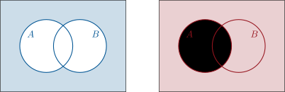
We take the notion of set and the membership relation $x \in E$ as primitive. For sets $A, B$ inside an ambient set $E$ :

inclusion: $A \subseteq B$ when $\forall x,\ x \in A \implies x \in B$ ; equality $A = B$ when $A \subseteq B$ and $B \subseteq A$ ;
union $A \cup B$ , intersection $A \cap B$ , difference $A \setminus B = \{x \in A : x \notin B\}$ , complement $\overline{A} = E \setminus A$ ;
the empty set $\emptyset$ , contained in every set;
the power set $\mathcal{P}(E)$ : the set of all subsets of $E$ ;
the product $E \times F$ : the set of ordered pairs $(x, y)$ with $x \in E$ , $y \in F$ .

Example 1.17 (Getting used to the power set)

For $E = \{a, b\}$ :

\mathcal P(E) = \bigl\{\, \emptyset,\ \{a\},\ \{b\},\ \{a, b\} \,\bigr\},

four elements — and note the type discipline: $a \in E$ but $\{a\} \in \mathcal P(E)$ ; the statements $a \in \mathcal P(E)$ and $\{a\} \subseteq \mathcal P(E)$ are both false as written (the second would require $a$ to be a subset of $E$ ). Iterating from nothing: $\mathcal P(\emptyset) = \{\emptyset\}$ has one element, $\mathcal P(\mathcal P(\emptyset)) = \{\emptyset, \{\emptyset\}\}$ has two, the next has four — sets of sets are ordinary sets, and Chapter 2 will confirm the doubling pattern: $\abs{\mathcal P(E)} = 2^{\abs E}$ . Keeping the levels ( $x$ , $\{x\}$ , $\{\{x\}\}$ ) straight is half the battle in exercises like Exercises 1.11 and 1.12.

Proposition 1.18 (Set algebra)

For subsets $A, B, C$ of $E$ :

$A \cap (B \cup C) = (A \cap B) \cup (A \cap C)$ and $A \cup (B \cap C) = (A \cup B) \cap (A \cup C)$ ;
De Morgan: $\overline{A \cup B} = \overline{A} \cap \overline{B}$ and $\overline{A \cap B} = \overline{A} \cup \overline{B}$ ;
$A \subseteq B \iff \overline{B} \subseteq \overline{A}$ .

Proof. Each identity translates a rule of Proposition 1.3 through the dictionary ( $\in A$ or not) $\leftrightarrow$ (statement true or false): e.g. $x \in \overline{A \cup B} \iff \lnot(x \in A \lor x \in B) \iff (x \notin A) \land (x \notin B) \iff x \in \overline{A} \cap \overline{B}$ . Point (3) is contraposition. As a second sample, the first distributivity law in full:

x \in A \cap (B \cup C) \iff (x \in A) \land \bigl(x \in B \lor x \in C\bigr) \iff \bigl(x \in A \land x \in B\bigr) \lor \bigl(x \in A \land x \in C\bigr),

by the distributivity of Proposition 1.3 (6), and the last statement reads $x \in (A \cap B) \cup (A \cap C)$ . Every set identity of this kind is provable by this one mechanical translation — which is why none of them needs memorizing. ∎

Method 1.19 (Proving set equalities)

To prove $A = B$ , prove the two inclusions: let $x \in A$ , show $x \in B$ ; then let $x \in B$ , show $x \in A$ . Alternatively, chain equivalences $x \in A \iff \dots \iff x \in B$ when each step really is an equivalence.

De Morgan’s laws in pictures: the shaded region on the left is A ∪ B = A ∩ B (everything outside both disks); on the right, A ∩ B = A ∪ B (everything except the lens-shaped overlap). A diagram is not a proof, but it makes the element-chasing proof of impossible to misremember. — De Morgan’s laws in pictures: the shaded region on the left is $\overline{A \cup B} = \overline A \cap \overline B$ (everything outside both disks); on the right, $\overline{A \cap B} = \overline A \cup \overline B$ (everything except the lens-shaped overlap). A diagram is not a proof, but it makes the element-chasing proof of Proposition 1.18 impossible to misremember.

1.5 Maps

Definition 1.20 (Map, image, preimage)

A map (or function) $f \colon E \to F$ assigns to every element $x$ of the set $E$ (the domain) exactly one element $f(x)$ of the set $F$ (the codomain). For $A \subseteq E$ and $B \subseteq F$ :

f(A) = \{f(x) : x \in A\} \subseteq F, \qquad f^{-1}(B) = \{x \in E : f(x) \in B\} \subseteq E

are the direct image of $A$ and the preimage of $B$ . The composition of $f \colon E \to F$ and $g \colon F \to G$ is $g \circ f \colon E \to G$ , $x \mapsto g(f(x))$ .

Remark 1.21

The notation $f^{-1}(B)$ does not presuppose an inverse map: $f^{-1}(B)$ is defined for every $f$ . Preimages behave better than images: $f^{-1}$ preserves unions, intersections and complements, whereas $f(A \cap A') \subseteq f(A) \cap f(A')$ can be strict (Exercise 1.8).

Example 1.22 (Computing images and preimages)

Let $f \colon \R \to \R$ , $x \mapsto x^2$ . Then:

f\bigl(\intcc{-1}{2}\bigr) = \intcc04, \qquad f^{-1}\bigl(\intcc14\bigr) = \intcc{-2}{-1} \cup \intcc12, \qquad f^{-1}(\{-1\}) = \emptyset .

For the first: every $x \in \intcc{-1}2$ has $x^2 \in \intcc04$ , and every $y \in \intcc04$ is attained as $y = (\sqrt y)^2$ with $\sqrt y \in \intcc02 \subseteq \intcc{-1}2$ — note that the image is not $\intcc14 = \{(-1)^2, 2^2\}$ : images of intervals are not computed from endpoints alone. For the second: $1 \leq x^2 \leq 4 \iff 1 \leq \abs x \leq 2$ , which splits into two pieces. The third illustrates that a preimage may be empty — $f^{-1}(B)$ always makes sense, however small the intersection of $B$ with the image. Finally observe on this example the strictness phenomenon of the remark above: with $A = \intcc{-1}0$ and $A' = \intcc01$ , one has $f(A \cap A') = f(\{0\}) = \{0\}$ , while $f(A) \cap f(A') = \intcc01$ .

Definition 1.23 (Injective, surjective, bijective)

A map $f \colon E \to F$ is:

injective when distinct elements have distinct images: $\forall x, x' \in E,\ f(x) = f(x') \implies x = x'$ ;
surjective when every element of $F$ is attained: $\forall y \in F,\ \exists x \in E,\ f(x) = y$ ;
bijective when it is both, i.e. every $y \in F$ has exactly one preimage.

Theorem 1.24 (Inverse map)

A map $f \colon E \to F$ is bijective if and only if there is a map $g \colon F \to E$ with $g \circ f = \mathrm{id}_E$ and $f \circ g = \mathrm{id}_F$ . In that case $g$ is unique; it is written $f^{-1}$ and called the inverse of $f$ , and $f^{-1}$ is itself bijective with $(f^{-1})^{-1} = f$ .

Proof. ( $\Rightarrow$ ) If $f$ is bijective, every $y \in F$ has a unique preimage; define $g(y)$ to be that preimage. Then $f(g(y)) = y$ by construction, and $g(f(x)) = x$ because $x$ is the preimage of $f(x)$ .

( $\Leftarrow$ ) Suppose such a $g$ exists. If $f(x) = f(x')$ , applying $g$ gives $x = x'$ : $f$ is injective. For $y \in F$ , $x = g(y)$ satisfies $f(x) = y$ : $f$ is surjective.

Uniqueness: if $g$ and $h$ both work, then $g = g \circ \mathrm{id}_F = g \circ (f \circ h) = (g \circ f) \circ h = h$ . Finally the pair of identities is symmetric in $f$ and $g$ , so $g = f^{-1}$ is bijective with inverse $f$ . ∎

Example 1.25 (Computing an inverse in practice)

Let $f \colon \R \to \intoo0{+\infty}$ , $f(x) = \eu^{2x+1}$ . To invert, solve $y = f(x)$ for a given $y > 0$ :

y = \eu^{2x+1} \iff \ln y = 2x + 1 \iff x = \frac{\ln y - 1}2 ,

each step being reversible on the announced domains. The computation delivers everything at once: for each $y$ in the codomain there is exactly one solution $x$ , so $f$ is bijective, and

f^{-1} \colon \intoo0{+\infty} \to \R, \qquad f^{-1}(y) = \frac{\ln y - 1}2 .

A quick check of both compositions ( $f^{-1}(f(x)) = \frac{(2x+1) - 1}2 = x$ and $f(f^{-1}(y)) = \eu^{\ln y} = y$ ) confirms Theorem 1.24’s criterion. The insight: “solve for $x$ and watch the equivalences” is simultaneously the existence proof, the uniqueness proof, and the formula — but it only works if the codomain was announced correctly ( $f$ is not surjective onto $\R$ ).

Proposition 1.26 (Composition and the three properties)

Let $f \colon E \to F$ and $g \colon F \to G$ .

If $f$ and $g$ are injective (resp. surjective, bijective), so is $g \circ f$ ; and then $(g \circ f)^{-1} = f^{-1} \circ g^{-1}$ in the bijective case.
If $g \circ f$ is injective, then $f$ is injective. If $g \circ f$ is surjective, then $g$ is surjective.

Proof. (1) If $g(f(x)) = g(f(x'))$ , injectivity of $g$ gives $f(x) = f(x')$ , then injectivity of $f$ gives $x = x'$ . If $z \in G$ , surjectivity of $g$ gives $y$ with $g(y) = z$ , then surjectivity of $f$ gives $x$ with $f(x) = y$ , so $g(f(x)) = z$ . In the bijective case one checks directly that $f^{-1} \circ g^{-1}$ is a two-sided inverse of $g \circ f$ , and uniqueness in Theorem 1.24 concludes.

(2) If $f(x) = f(x')$ then $g(f(x)) = g(f(x'))$ , and injectivity of $g \circ f$ gives $x = x'$ . If $z \in G$ , surjectivity of $g \circ f$ gives $x$ with $g(f(x)) = z$ : then $y = f(x)$ satisfies $g(y) = z$ . ∎

Example 1.27 (Point (2) is sharp)

In Proposition 1.26 (2), one cannot upgrade the conclusions: $g \circ f$ bijective does not force $f$ surjective or $g$ injective. Take $E = G = \{1\}$ , $F = \{1, 2\}$ , with $f(1) = 1$ and $g(1) = g(2) = 1$ : then $g \circ f = \mathrm{id}_E$ is bijective, yet $f$ misses the element $2$ and $g$ collapses both elements. The moral is a precise bookkeeping rule: composition information flows to the inner map for injectivity and to the outer map for surjectivity, never the other way. (Exercise 1.9 builds the same phenomenon with infinite sets, where it is the engine behind one-sided inverses.)

Example 1.28

$f \colon \R \to \R$ , $x \mapsto x^2$ is neither injective ( $f(-1) = f(1)$ ) nor surjective ( $-1$ has no preimage). Restricting the domain and codomain, $f \colon \R_+ \to \R_+$ , $x \mapsto x^2$ is bijective, with inverse $y \mapsto \sqrt y$ . A map’s injectivity or surjectivity depends on the announced domain and codomain, not only on the formula.

1.6 Relations

Definition 1.29 (Equivalence relation)

A binary relation $\mathcal{R}$ on a set $E$ is an equivalence relation when it is: reflexive ( $x \mathbin{\mathcal{R}} x$ for all $x$ ), symmetric ( $x \mathbin{\mathcal{R}} y \implies y \mathbin{\mathcal{R}} x$ ) and transitive ( $x \mathbin{\mathcal{R}} y$ and $y \mathbin{\mathcal{R}} z$ imply $x \mathbin{\mathcal{R}} z$ ). The equivalence class of $x$ is $\mathrm{cl}(x) = \{y \in E : x \mathbin{\mathcal{R}} y\}$ .

Example 1.30 (Checking the three axioms)

On $\R$ , declare $x \mathbin{\mathcal{R}} y$ when $x - y \in \Z$ . Reflexive: $x - x = 0 \in \Z$ . Symmetric: if $x - y \in \Z$ then $y - x = -(x - y) \in \Z$ . Transitive: if $x - y \in \Z$ and $y - z \in \Z$ , then $x - z = (x - y) + (y - z) \in \Z$ (a sum of integers). So $\mathcal R$ is an equivalence relation, and $\mathrm{cl}(x) = x + \Z = \{x + k : k \in \Z\}$ : each class contains exactly one representative in $\intco01$ , its fractional part. By contrast, the relation “ $\abs{x - y} \leq 1$ ” on $\R$ is reflexive and symmetric but not transitive ( $0 \mathbin{\mathcal R} 1$ and $1 \mathbin{\mathcal R} 2$ , yet $\abs{0 - 2} > 1$ ): closeness does not propagate, and no partition into classes exists — a useful counterexample to keep in mind when verifying the axioms feels routine.

Theorem 1.31 (Classes form a partition)

Let $\mathcal{R}$ be an equivalence relation on $E$ . Then the equivalence classes are nonempty, pairwise disjoint or equal, and their union is $E$ : they form a partition of $E$ . Conversely, every partition of $E$ arises this way from exactly one equivalence relation (“being in the same piece”).

Proof. $x \in \mathrm{cl}(x)$ by reflexivity, so classes are nonempty with union $E$ . Suppose $\mathrm{cl}(x) \cap \mathrm{cl}(y) \neq \emptyset$ , say $z$ lies in both. Then $x \mathbin{\mathcal{R}} z$ and $y \mathbin{\mathcal{R}} z$ , so by symmetry and transitivity $x \mathbin{\mathcal{R}} y$ . Now for any $t \in \mathrm{cl}(y)$ , transitivity gives $t \in \mathrm{cl}(x)$ , and symmetrically: the two classes are equal. For the converse, let $(E_i)_{i \in I}$ be a partition of $E$ and define $x \mathbin{\mathcal S} y$ to mean “some piece contains both $x$ and $y$ ”. Reflexive: $x$ lies in some piece, which then contains $x$ twice over. Symmetric: the defining condition is symmetric in $x$ and $y$ . Transitive: if $x, y \in E_i$ and $y, z \in E_j$ , then $y \in E_i \cap E_j$ , so $E_i = E_j$ (distinct pieces are disjoint) and $x, z$ share a piece. The $\mathcal S$ -class of $x$ is exactly the piece containing $x$ , so the classes are the given pieces. Finally the relation is determined by its classes: two equivalence relations with the same classes relate the same pairs, since each relates $x$ and $y$ exactly when $y$ belongs to the class of $x$ — whence the uniqueness claim. ∎

Example 1.32

On $\Z$ , congruence modulo $n$ ( $x \equiv y \pmod n$ when $n$ divides $x - y$ ) is an equivalence relation; its classes are the $n$ sets of integers with a given remainder upon division by $n$ . This example becomes the ring $\Z/n\Z$ in Chapter 7.

Definition 1.33 (Order relation)

A relation $\preceq$ on $E$ is an order when it is reflexive, antisymmetric ( $x \preceq y$ and $y \preceq x$ imply $x = y$ ) and transitive. The order is total when any two elements are comparable, partial otherwise. An element $M \in A \subseteq E$ is a greatest element of $A$ when $a \preceq M$ for all $a \in A$ ; greatest (and least) elements are unique when they exist.

Example 1.34

$(\R, \leq)$ is totally ordered. $(\mathcal{P}(E), \subseteq)$ is partially ordered as soon as $E$ has two elements: $\{a\}$ and $\{b\}$ are not comparable. The subset $A = \{\{a\}, \{b\}\}$ of $\mathcal{P}(\{a,b\})$ has no greatest element, yet has an upper bound $\{a, b\}$ : the distinction between greatest elements and upper bounds returns, for $\R$ , in Chapter 10.

Example 1.35 (Two orders on the grid $\N^2$ )

On pairs of naturals, compare componentwise: $(a, b) \preceq (a', b')$ when $a \leq a'$ and $b \leq b'$ (the product order). This is an order — each axiom is inherited coordinate by coordinate — but a partial one: $(1, 3)$ and $(2, 0)$ are incomparable. Now compare like a dictionary: $(a, b) \preceq_{\mathrm{lex}} (a', b')$ when $a < a'$ , or $a = a'$ and $b \leq b'$ (the lexicographic order). Transitivity requires a two-case check but holds, and any two pairs are now comparable: the order is total. The two orders rank the same set differently — $(0, 100) \preceq_{\mathrm{lex}} (1, 0)$ though the product order says nothing — a reminder that an order is a structure one chooses, not a property of the set. Lexicographic comparison is also the standard trick for turning several sorting criteria into one.

Remark 1.36 (Interlude: size as bijection)

A quiet theme of this chapter deserves a spotlight: bijections are the mathematician’s notion of “same size”. For finite sets this becomes the counting calculus of Chapter 2, where every formula is secretly a bijection; for infinite sets it becomes the weekend problem below, where $\N$ , $\Q$ and $\R$ turn out to have genuinely different sizes. The same dictionary reappears twice more in this volume in refined forms: sequences (Chapter 11) are nothing but maps $\N \to \R$ , so statements about sequences are statements about a set of maps; and linear algebra will measure vector spaces not by bijections but by linear bijections, whose existence is governed by a single number, the dimension (Chapter 19). Whenever a new “sameness” appears — equipotence, isomorphism of groups (Chapter 7), linear isomorphism — the pattern of Theorem 1.24 repeats: sameness is an invertible, structure-respecting map.

Remark 1.37 (Where this chapter is used)

Everywhere — but a few places deserve flagging. The three-quantifier gymnastics of Example 1.8 is the daily bread of Chapters 11 and 13: every limit proof is a game played against an arbitrary $\varepsilon$ . Equivalence classes reappear as the congruence classes of $\Z/n\Z$ in Chapter 7, where the partition of Theorem 1.31 acquires an algebraic structure of its own. Order relations, upper bounds and least upper bounds become the axiomatic heart of $\R$ in Chapter 10. Injections, surjections and bijections return as the linear maps of Chapter 20, where injectivity can be tested on a single vector (the kernel); and the weekend problem below turns the bare notion of bijection into a theory of the sizes of infinite sets, whose conclusions (countability of $\Q$ , uncountability of $\R$ ) resurface in Chapters 10 and 12.

1.7 Exercises

Exercise 1.1 ★

Write the negation of each statement, without using the word “not”:

$\forall x \in \R,\ \exists y \in \R,\ x + y > 0$ ;
$\exists x \in \R,\ \forall y \in \R,\ xy = 0$ ;
$\forall \varepsilon > 0,\ \exists \delta > 0,\ \forall x \in \R,\ \abs{x} \leq \delta \implies \abs{f(x)} \leq \varepsilon$ (for a fixed map $f \colon \R \to \R$ ).

Then decide whether statements (1) and (2) are true.

Solution

Solution of Exercise 1.1.

Negations, pushing $\lnot$ through each quantifier (Proposition 1.5) and using $\lnot(P \implies Q) \iff P \land \lnot Q$ :

$\exists x \in \R,\ \forall y \in \R,\ x + y \leq 0$ ;
$\forall x \in \R,\ \exists y \in \R,\ xy \neq 0$ ;
$\exists \varepsilon > 0,\ \forall \delta > 0,\ \exists x \in \R,\ \abs{x} \leq \delta \text{ and } \abs{f(x)} > \varepsilon$ .

Statement (1) is true: given $x$ , take $y = -x + 1$ ; then $x + y = 1 > 0$ . Statement (2) is true: $x = 0$ satisfies $xy = 0$ for all $y$ .

Exercise 1.2 ★

Let $P, Q$ be statements. Using truth tables, prove that $\lnot(P \implies Q) \iff P \land (\lnot Q)$ , and deduce the negation of: “if a function is differentiable then it is continuous”.

Solution

Solution of Exercise 1.2.

Truth table, writing T/F for the four cases $(P, Q)$ :

$P$	$Q$	$P \implies Q$	$\lnot(P \implies Q)$	$\lnot Q$	$P \land \lnot Q$
T	T	T	F	F	F
T	F	F	T	T	T
F	T	T	F	F	F
F	F	T	F	T	F

Columns $4$ and $6$ coincide, proving the equivalence. The negation of “if a function is differentiable then it is continuous” is therefore: “there is a function which is differentiable and not continuous” (a false statement, as it happens: the original implication is true, see Chapter 14).

Exercise 1.3 ★

Prove by contraposition: for $x \in \R$ , if $x^3 + x \geq 2$ then $x \geq 1$ . Then prove by contradiction: there is no smallest strictly positive real number.

Solution

Solution of Exercise 1.3.

Contraposition. Assume $x < 1$ . Then $x^3 < 1$ (the cube function is increasing) and $x < 1$ , so $x^3 + x < 2$ . This proves the contrapositive, hence the statement.

Contradiction. Suppose $a > 0$ is the smallest strictly positive real. Then $a/2$ is strictly positive and $a/2 < a$ (since $a > 0$ ), contradicting minimality. Hence no such $a$ exists.

Exercise 1.4 ★

Prove by induction that for all $n \in \N$ :

$\sum_{k=0}^{n} 2^k = 2^{n+1} - 1$ ;
$4^n + 5$ is divisible by $3$ .

Solution

Solution of Exercise 1.4.

Base case $n = 0$ : $2^0 = 1 = 2^1 - 1$ . Step: assuming the identity for $n$ ,

$\sum_{k=0}^{n+1} 2^k = (2^{n+1} - 1) + 2^{n+1} = 2 \cdot 2^{n+1} - 1 = 2^{n+2} - 1 .$
Base case $n = 0$ : $4^0 + 5 = 6 = 3 \times 2$ . Step: if $4^n + 5 = 3m$ , then

$4^{n+1} + 5 = 4(4^n + 5) - 15 = 3(4m - 5),$

divisible by $3$ .

Exercise 1.5 ★

Find the flaw in the following “proof” that all pencils have the same color. Let $P(n)$ : “in every set of $n$ pencils, all pencils have the same color”. $P(1)$ is clear. Assume $P(n)$ and take $n+1$ pencils; removing the last one, the first $n$ share their color; removing the first one, the last $n$ share their color; hence all $n+1$ share their color.

Solution

Solution of Exercise 1.5.

The inductive step silently assumes that the two groups (“the first $n$ ” and “the last $n$ ”) overlap, so that the shared pencils carry the color from one group to the other. For $n + 1 = 2$ the two groups are $\{$ first pencil $\}$ and $\{$ second pencil $\}$ : they are disjoint, and the argument breaks. So $P(1) \implies P(2)$ was never proved, and the induction collapses — even though $P(n) \implies P(n+1)$ is valid for every $n \geq 2$ .

Exercise 1.6 ★

Let $A, B, C$ be subsets of $E$ . Prove:

$A \setminus B = A \cap \overline{B}$ ;
$(A \cup B) \setminus C = (A \setminus C) \cup (B \setminus C)$ ;
$A \subseteq B \iff A \cup B = B \iff A \cap B = A$ .

Solution

Solution of Exercise 1.6.

$x \in A \setminus B \iff x \in A \land x \notin B \iff x \in A \land x \in \overline{B} \iff x \in A \cap \overline{B}$ .
Using (1) and distributivity (Proposition 1.18): $(A \cup B) \cap \overline{C} = (A \cap \overline{C}) \cup (B \cap \overline{C})$ .
Suppose $A \subseteq B$ . Then $A \cup B \subseteq B$ (both pieces lie in $B$ ) and $B \subseteq A \cup B$ always, so $A \cup B = B$ . Suppose $A \cup B = B$ : then $A \cap B \subseteq A$ always, and $A \subseteq A \cup B = B$ gives $A \subseteq A \cap B$ , so $A \cap B = A$ . Suppose $A \cap B = A$ : then $A = A \cap B \subseteq B$ . The three conditions are thus equivalent (we proved a cycle of implications).

Exercise 1.7 ★★

For each map, decide (with proof) whether it is injective, surjective, bijective:

$f \colon \N \to \N$ , $n \mapsto n + 1$ ;
$g \colon \Z \to \Z$ , $n \mapsto n + 1$ ;
$h \colon \R \setminus \{1\} \to \R$ , $x \mapsto \frac{x+1}{x-1}$ .

For $h$ , adjust the codomain to make it bijective and compute the inverse.

Solution

Solution of Exercise 1.7.

$f$ is injective ( $n + 1 = m + 1 \implies n = m$ ) but not surjective: $0$ has no preimage in $\N$ .
$g$ is bijective: $n \mapsto n - 1$ is a two-sided inverse on $\Z$ .
$h$ is injective: $\frac{x+1}{x-1} = \frac{x'+1}{x'-1}$ gives $(x+1)(x'-1) = (x'+1)(x-1)$ , i.e. $xx' - x + x' - 1 = xx' - x' + x - 1$ , so $2x' = 2x$ . It is not surjective onto $\R$ : solving $y = \frac{x+1}{x-1}$ gives $x(y - 1) = y + 1$ , which has no solution when $y = 1$ (the equation reads $0 = 2$ ). With codomain $\R \setminus \{1\}$ , the same computation gives the unique preimage $x = \frac{y+1}{y-1}$ , so $h \colon \R \setminus \{1\} \to \R \setminus \{1\}$ is bijective and $h^{-1}(y) = \frac{y+1}{y-1} = h(y)$ : $h$ is its own inverse.

Exercise 1.8 ★★

Let $f \colon E \to F$ , let $A, A' \subseteq E$ and $B, B' \subseteq F$ .

Prove $f^{-1}(B \cap B') = f^{-1}(B) \cap f^{-1}(B')$ and $f(A \cup A') = f(A) \cup f(A')$ .
Prove $f(A \cap A') \subseteq f(A) \cap f(A')$ and give an example where the inclusion is strict.
Prove: $f$ is injective if and only if $f(A \cap A') = f(A) \cap f(A')$ for all $A, A'$ .

Solution

Solution of Exercise 1.8.

$x \in f^{-1}(B \cap B') \iff f(x) \in B \cap B' \iff f(x) \in B \land f(x) \in B' \iff x \in f^{-1}(B) \cap f^{-1}(B')$ . For images: $y \in f(A \cup A')$ iff $y = f(x)$ for some $x$ in $A$ or in $A'$ , iff $y \in f(A)$ or $y \in f(A')$ .
If $y \in f(A \cap A')$ , then $y = f(x)$ with $x \in A$ and $x \in A'$ , so $y \in f(A)$ and $y \in f(A')$ . Strictness: take $f \colon \R \to \R$ , $x \mapsto x^2$ , $A = \{-1\}$ , $A' = \{1\}$ : then $f(A \cap A') = f(\emptyset) = \emptyset$ but $f(A) \cap f(A') = \{1\}$ .
( $\Leftarrow$ ) With $A = \{x\}$ , $A' = \{x'\}$ for $x \neq x'$ : if $f(x) = f(x')$ , then $f(A) \cap f(A') = \{f(x)\}$ while $f(A \cap A') = \emptyset$ , contradicting the assumed equality; so $f$ is injective. ( $\Rightarrow$ ) Let $f$ be injective and $y \in f(A) \cap f(A')$ : $y = f(x) = f(x')$ with $x \in A$ , $x' \in A'$ ; injectivity gives $x = x' \in A \cap A'$ , so $y \in f(A \cap A')$ . With (2), equality holds.

Exercise 1.9 ★★

Let $f \colon E \to F$ and $g \colon F \to E$ satisfy $g \circ f = \mathrm{id}_E$ . Prove that $f$ is injective and $g$ is surjective. Give an example where neither $f$ nor $g$ is bijective.

Solution

Solution of Exercise 1.9.

$g \circ f = \mathrm{id}_E$ is injective and surjective, so by Proposition 1.26 (2), $f$ is injective and $g$ is surjective. Example: $E = \N$ , $F = \Z$ , $f$ the inclusion $n \mapsto n$ , and $g \colon \Z \to \N$ , $g(n) = n$ for $n \geq 0$ and $g(n) = 0$ for $n < 0$ . Then $g(f(n)) = n$ for all $n \in \N$ , but $f$ is not surjective and $g$ is not injective.

Exercise 1.10 ★★

On $\R$ , define $x \mathbin{\mathcal{R}} y \iff x^2 - y^2 = x - y$ . Prove that $\mathcal{R}$ is an equivalence relation and describe the equivalence class of each real $x$ . Which classes have exactly one element?

Solution

Solution of Exercise 1.10.

$x^2 - y^2 = x - y \iff (x - y)(x + y) = x - y \iff (x - y)(x + y - 1) = 0 \iff y = x$ or $y = 1 - x$ . Reflexive: $y = x$ works. Symmetric: the condition “ $y = x$ or $y = 1 - x$ ” is symmetric in $x$ and $y$ (if $y = 1 - x$ then $x = 1 - y$ ). Transitive: suppose $x \mathbin{\mathcal{R}} y$ and $y \mathbin{\mathcal{R}} z$ ; going through the four cases, $z$ equals $x$ or $1 - x$ each time (e.g. $y = 1 - x$ and $z = 1 - y$ give $z = x$ ). So $\mathcal{R}$ is an equivalence relation and $\mathrm{cl}(x) = \{x,\, 1 - x\}$ . This class has one element exactly when $x = 1 - x$ , i.e. for $x = \frac12$ .

Exercise 1.11 ★★★

(Cantor) Let $E$ be a set. Prove that there is no surjection from $E$ onto $\mathcal{P}(E)$ . Hint: given $f \colon E \to \mathcal{P}(E)$ , consider $D = \{x \in E : x \notin f(x)\}$ .

Solution

Solution of Exercise 1.11.

Let $f \colon E \to \mathcal{P}(E)$ be any map and set $D = \{x \in E : x \notin f(x)\} \in \mathcal{P}(E)$ . Suppose $D = f(a)$ for some $a \in E$ . If $a \in D$ , then by definition of $D$ , $a \notin f(a) = D$ : contradiction. If $a \notin D$ , then $a \notin f(a)$ , so by definition of $D$ , $a \in D$ : contradiction. Hence $D$ is not in the image of $f$ , and $f$ is not surjective. (In particular no set is in bijection with its power set: there are “more” subsets of $\N$ than integers.)

Exercise 1.12 ★★★

Let $f \colon E \to F$ be a map. Define $\Phi \colon \mathcal{P}(F) \to \mathcal{P}(E)$ by $\Phi(B) = f^{-1}(B)$ .

Prove that $f$ is surjective if and only if $\Phi$ is injective.
Prove that $f$ is injective if and only if $\Phi$ is surjective.

Solution

Solution of Exercise 1.12.

( $\Rightarrow$ ) Let $f$ be surjective and $\Phi(B) = \Phi(B')$ . For $y \in B$ , pick $x$ with $f(x) = y$ ; then $x \in f^{-1}(B) = f^{-1}(B')$ , so $y = f(x) \in B'$ . Hence $B \subseteq B'$ , and symmetrically $B' \subseteq B$ : $\Phi$ is injective. ( $\Leftarrow$ ) If $f$ is not surjective, pick $y_0 \in F$ outside the image; then $f^{-1}(\{y_0\}) = \emptyset = f^{-1}(\emptyset)$ with $\{y_0\} \neq \emptyset$ , so $\Phi$ is not injective.
( $\Rightarrow$ ) Let $f$ be injective and $A \subseteq E$ . Set $B = f(A)$ ; then $f^{-1}(B) = \{x : f(x) \in f(A)\}$ , and injectivity gives $f(x) \in f(A) \iff x \in A$ , so $\Phi(B) = A$ : $\Phi$ is surjective. ( $\Leftarrow$ ) If $f$ is not injective, take $x \neq x'$ with $f(x) = f(x')$ . Every preimage set $f^{-1}(B)$ contains $x$ if and only if it contains $x'$ ; hence $\{x\}$ is not of the form $\Phi(B)$ , and $\Phi$ is not surjective.

1.8 Problem: Comparing infinities

Problem 1.1

When do two sets have “the same number of elements”? Cantor’s answer — when there is a bijection between them — turns out to be usable even for infinite sets, and it splits infinity into genuinely different sizes. This problem builds the whole toolbox from the bare definitions of this chapter: the Cantor–Schröder–Bernstein theorem (two injections manufacture a bijection), the countability of $\Q$ , the uncountability of $\R$ by the diagonal argument, and Cantor’s astonishing 1874 conclusion: transcendental numbers exist, and massively so, without exhibiting a single one. Throughout, for sets $E$ and $F$ , write $E \preceq F$ when there exists an injection from $E$ into $F$ , and $E \approx F$ (“ $E$ and $F$ are equipotent”) when there exists a bijection from $E$ onto $F$ .

Part I — The vocabulary of comparison.

Show that $\approx$ behaves like an equivalence relation: $E \approx E$ ; if $E \approx F$ then $F \approx E$ ; if $E \approx F$ and $F \approx G$ then $E \approx G$ . (Quote precisely Theorem 1.24 and Proposition 1.26.)
Show that $\preceq$ is transitive, and that an injection $f \colon E \to F$ always induces $E \approx f(E)$ .
Let $E \neq \emptyset$ . Show that $E \preceq F$ if and only if there exists a surjection from $F$ onto $E$ .
Verify that $n \mapsto n + 1$ is a bijection from $\N$ onto $\N^* = \N \setminus \{0\}$ , and that

$\sigma(n) = \frac n2 \ \ (n \text{ even}), \qquad \sigma(n) = -\frac{n+1}2 \ \ (n \text{ odd})$

is a bijection from $\N$ onto $\Z$ . Hence removing a point, or doubling into negatives, does not change the size of $\N$ .

Part II — The Cantor–Schröder–Bernstein theorem. Let $f \colon E \to F$ and $g \colon F \to E$ be two injections. Define

C_0 = E \setminus g(F), \qquad C_{n+1} = g\bigl(f(C_n)\bigr) \ \ (n \in \N), \qquad C = \bigcup_{n \in \N} C_n,

and let $h \colon E \to F$ send $x \in C$ to $f(x)$ , and $x \notin C$ to the unique $y \in F$ with $g(y) = x$ .

Check that $h$ is well defined: if $x \notin C$ then $x \in g(F)$ , and the element $y$ with $g(y) = x$ is unique.
Show that $g\bigl(f(C)\bigr) = \bigcup_{n \geq 1} C_n \subseteq C$ . (Direct images commute with unions: Exercise 1.8.)
Show that $h$ is injective. (Three cases; in the mixed case $x \in C$ , $x' \notin C$ , show that $h(x) = h(x')$ would force $x' \in g(f(C)) \subseteq C$ .)
Show that $h$ is surjective: given $y \in F$ , distinguish the cases $g(y) \notin C$ and $g(y) \in C_n$ for some $n \geq 1$ (why is $g(y) \in C_0$ impossible?), and exhibit a preimage of $y$ in each case.
Conclude with the Cantor–Schröder–Bernstein theorem: if $E \preceq F$ and $F \preceq E$ , then $E \approx F$ . Comment in one sentence on what makes this statement nontrivial.
Two applications. (a) Show $\intcc01 \approx \intoo01$ . (b) Show that $\varphi(p, q) = 2^p(2q + 1) - 1$ defines a bijection from $\N \times \N$ onto $\N$ — injectivity by a parity argument, surjectivity by strong induction (Theorem 1.12). Hence $\N \times \N \approx \N$ : the plane of integer points is no bigger than the line.

Part III — Countable sets. Call a set $E$ at most countable when $E \preceq \N$ , and countable when $E \approx \N$ .

Show that every infinite subset $A \subseteq \N$ is countable. (Define $\varphi(n)$ recursively as the least element of $A \setminus \{\varphi(0), \dots, \varphi(n-1)\}$ ; show $\varphi$ is strictly increasing, satisfies $\varphi(n) \geq n$ , and attains every element of $A$ .)
Deduce that a set is at most countable if and only if it is finite or countable, and observe that question 9 gives the shortcut: if $E \preceq \N$ and $\N \preceq E$ , then $E$ is countable.
Show that if $E$ and $F$ are at most countable, so is $E \times F$ . Deduce that $\Z \times \N^*$ is countable.
Show that $\Q$ is countable. (Inject $\Q$ into $\Z \times \N^*$ by writing each rational in lowest terms with positive denominator — the uniqueness of that representation is proved in Chapter 6; then apply question 12.)
Show that a countable union of at most countable sets is at most countable: if each $E_n$ ( $n \in \N$ ) is at most countable, so is $\bigcup_{n \in \N} E_n$ . (Send $x$ to the pair $(n, f_n(x))$ where $n$ is the least index with $x \in E_n$ .)
Show that the set of finite subsets of $\N$ is countable. (Map a finite subset $F$ to $\sum_{i \in F} 2^i$ ; prove injectivity by comparing the largest element where two finite sets differ, using $\sum_{k=0}^{m-1} 2^k = 2^m - 1$ from Exercise 1.4.)

Part IV — Diagonalization. Let $\{0,1\}^{\N}$ denote the set of all maps $u \colon \N \to \{0, 1\}$ , i.e. the set of binary sequences.

Construct a bijection between $\mathcal{P}(\N)$ and $\{0,1\}^{\N}$ (indicator functions).
(The diagonal argument) Let $\Phi \colon \N \to \{0,1\}^{\N}$ be any map. Consider the sequence $d$ defined by $d(n) = 1 - \Phi(n)(n)$ . Show that $d$ is not in the image of $\Phi$ , and conclude that $\{0,1\}^{\N}$ is not at most countable. Explain in one sentence why, through question 17, this is exactly Cantor’s theorem (Exercise 1.11) for $E = \N$ .
Admit — as familiar from school, and established rigorously in Chapter 10 — that every $x \in \intco01$ has a unique proper decimal expansion $x = 0.d_1 d_2 d_3\dots$ (one not ending in an infinite string of $9$ s). Given any sequence $(x_n)_{n \geq 1}$ of elements of $\intco01$ , construct $x \in \intco01$ with $x \neq x_n$ for all $n$ : choose its $n$ -th digit to be $5$ if the $n$ -th digit of $x_n$ differs from $5$ , and $6$ otherwise. Justify carefully that $x$ is proper and avoids every $x_n$ , and conclude that $\intco01$ is not at most countable.
Deduce that $\R$ is uncountable, and that the set $\R \setminus \Q$ of irrational numbers is uncountable as well. In what precise sense are “most” real numbers irrational?

Part V — Cantor’s 1874 theorem: transcendental numbers exist. A real number $x$ is algebraic when $P(x) = 0$ for some nonzero polynomial $P$ with integer coefficients, and transcendental otherwise. Admit for this part — it is proved in Chapter 8 — that a nonzero polynomial of degree $n$ has at most $n$ real roots.

Show that every rational number is algebraic, and find explicit polynomials with integer coefficients annihilating $\sqrt 2$ and $\sqrt 2 + \sqrt 3$ .
For fixed $n \in \N$ , show that the set of polynomials of degree at most $n$ with integer coefficients is countable. (Inject it into $\Z^{n+1}$ and induct on $n$ with question 13.)
Deduce that the set of all polynomials with integer coefficients is countable.
Prove Cantor’s theorem on algebraic numbers: the set $\mathcal{A}$ of algebraic real numbers is countable.
Conclude: transcendental real numbers exist, and the set of transcendental numbers is uncountable. Then take stock of the whole problem in a few sentences: the chain $\N \approx \Z \approx \Q \approx \mathcal{A}$ , the strict jump to $\R \approx$ (essentially) $\mathcal{P}(\N)$ , where each tool (Cantor–Schröder–Bernstein, countable unions, the diagonal) was decisive — and the philosophical punch of proving that uncountably many transcendental numbers exist without naming even one. (Proving a specific number such as $\pi$ transcendental is far harder and beyond this volume.)

Solution

Solution of Problem 1.1.

1. Reflexive: $\mathrm{id}_E$ is a bijection of $E$ onto itself. Symmetric: if $f \colon E \to F$ is bijective, Theorem 1.24 provides $f^{-1} \colon F \to E$ , itself bijective. Transitive: if $f \colon E \to F$ and $g \colon F \to G$ are bijections, Proposition 1.26 (1) says $g \circ f \colon E \to G$ is a bijection. (This is only “like” an equivalence relation: the collection of all sets is not itself a set, by the paradoxes that Exercise 1.11 hints at; the three properties are what matters.)

2. If $f \colon E \to F$ and $g \colon F \to G$ are injective, $g \circ f$ is injective by Proposition 1.26 (1): $E \preceq G$ . For the second point, corestrict $f$ to its image: the map $\tilde f \colon E \to f(E)$ , $x \mapsto f(x)$ , is surjective by construction of $f(E)$ and injective because $f$ is, hence bijective: $E \approx f(E)$ .

3. ( $\Rightarrow$ ) Let $f \colon E \to F$ be injective and fix $a \in E$ ( $E \neq \emptyset$ ). Define $s \colon F \to E$ by: $s(y)$ is the unique $x$ with $f(x) = y$ when $y \in f(E)$ (uniqueness by injectivity), and $s(y) = a$ otherwise. For every $x \in E$ , $s(f(x)) = x$ , so every $x$ is attained: $s$ is surjective. ( $\Leftarrow$ ) Let $s \colon F \to E$ be surjective. For each $x \in E$ choose one $y_x \in F$ with $s(y_x) = x$ , and set $u(x) = y_x$ . If $u(x) = u(x')$ then $x = s(u(x)) = s(u(x')) = x'$ : $u \colon E \to F$ is injective.

4. $n \mapsto n + 1$ maps $\N$ into $\N^*$ , is injective ( $n + 1 = m + 1 \implies n = m$ ) and surjective (every $m \geq 1$ is $(m - 1) + 1$ with $m - 1 \in \N$ ). For $\sigma$ : it maps even numbers $0, 2, 4, \dots$ to $0, 1, 2, \dots$ and odd numbers $1, 3, 5, \dots$ to $-1, -2, -3, \dots$ Injectivity: the even inputs land in $\N$ ( $\sigma(n) = n/2 \geq 0$ ) and the odd inputs land in the strictly negative integers ( $\sigma(n) = -(n+1)/2 \leq -1$ ), so a collision must happen within one parity class, where $\sigma$ is strictly monotonic ( $n/2 = m/2$ or $(n+1)/2 = (m+1)/2$ forces $n = m$ ). Surjectivity: $k \geq 0$ is $\sigma(2k)$ ; $k \leq -1$ is $\sigma(-2k - 1)$ with $-2k - 1 \geq 1$ odd. So $\N \approx \N^*$ and $\N \approx \Z$ .

5. $C_0 = E \setminus g(F) \subseteq C$ , so $x \notin C$ implies $x \notin C_0$ , i.e. $x \in g(F)$ : some $y \in F$ satisfies $g(y) = x$ . If also $g(y') = x$ , injectivity of $g$ gives $y' = y$ . Hence the second clause of the definition of $h$ picks out a unique, well-defined element $g^{-1}(x)$ .

6. Direct images commute with unions (Exercise 1.8 (1), applied to $f$ then to $g$ ):

g\bigl(f(C)\bigr) = g\Bigl(f\Bigl(\bigcup_{n \in \N} C_n\Bigr)\Bigr) = \bigcup_{n \in \N} g\bigl(f(C_n)\bigr) = \bigcup_{n \in \N} C_{n+1} = \bigcup_{n \geq 1} C_n \subseteq C .

7. Let $x \neq x'$ in $E$ . If both lie in $C$ , then $h(x) = f(x) \neq f(x') = h(x')$ by injectivity of $f$ . If neither lies in $C$ , then $g(h(x)) = x \neq x' = g(h(x'))$ , so $h(x) \neq h(x')$ . If $x \in C$ and $x' \notin C$ (the mixed case, up to swapping names): suppose $h(x) = h(x')$ , i.e. $f(x) = g^{-1}(x')$ . Applying $g$ : $x' = g(f(x)) \in g(f(C))$ , and question 6 gives $x' \in C$ — contradiction. So $h(x) \neq h(x')$ in all cases: $h$ is injective.

8. Let $y \in F$ . Case 1: $g(y) \notin C$ . Then $h(g(y)) = g^{-1}(g(y)) = y$ : the element $g(y)$ is a preimage. Case 2: $g(y) \in C$ , say $g(y) \in C_n$ . Since $g(y) \in g(F)$ , we have $g(y) \notin C_0 = E \setminus g(F)$ , so $n \geq 1$ and $g(y) \in C_n = g(f(C_{n-1}))$ : there is $x \in C_{n-1}$ with $g(y) = g(f(x))$ . Injectivity of $g$ gives $y = f(x)$ , and $x \in C_{n-1} \subseteq C$ , so $h(x) = f(x) = y$ . In both cases $y$ is attained: $h$ is surjective, hence bijective.

9. If $E \preceq F$ and $F \preceq E$ , pick injections $f \colon E \to F$ and $g \colon F \to E$ ; questions 5–8 build a bijection $h \colon E \to F$ , so $E \approx F$ . The statement is nontrivial because the two given injections are unrelated — neither need be surjective, and no formula mixing $f$ and $g$ naively defines a map: the whole content is the partition of $E$ into the region $C$ (where one copies $f$ ) and its complement (where one runs $g$ backwards).

10. (a) The inclusion $\intoo01 \to \intcc01$ is injective; and $x \mapsto \frac{x + 1}3$ maps $\intcc01$ injectively into $\intcc{\frac13}{\frac23} \subseteq \intoo01$ (it is affine with nonzero slope). By question 9, $\intcc01 \approx \intoo01$ — a bijection which is quite unpleasant to write down explicitly. (b) Injectivity. Suppose $2^p(2q + 1) = 2^{p'}(2q' + 1)$ with, say, $p \leq p'$ . Dividing by $2^p$ : $2q + 1 = 2^{p' - p}(2q' + 1)$ . If $p' > p$ the right side is even and the left side odd — impossible; so $p = p'$ , then $2q + 1 = 2q' + 1$ and $q = q'$ . Surjectivity. We show by strong induction that every integer $m \geq 1$ is of the form $2^p(2q + 1)$ . For $m = 1$ : $p = q = 0$ . Let $m \geq 1$ and assume the claim for all integers of $\intint1m$ . If $m + 1$ is odd, $m + 1 = 2q + 1$ with $p = 0$ . If $m + 1$ is even, $m + 1 = 2m'$ with $1 \leq m' \leq m$ ; by hypothesis $m' = 2^p(2q + 1)$ , so $m + 1 = 2^{p+1}(2q + 1)$ . Hence $\varphi(p, q) = 2^p(2q + 1) - 1$ hits every $n \in \N$ , and $\varphi$ is a bijection $\N \times \N \to \N$ .

11. Since $A$ is infinite, $A \setminus \{\varphi(0), \dots, \varphi(n - 1)\}$ is never empty, and the least-element property of $\N$ (used to prove Theorem 1.12) makes the recursive definition legitimate. Strictly increasing: $\varphi(n + 1)$ belongs to $A \setminus \{\varphi(0), \dots, \varphi(n)\} \subseteq A \setminus \{\varphi(0), \dots, \varphi(n - 1)\}$ , whose minimum is $\varphi(n)$ ; so $\varphi(n + 1) \geq \varphi(n)$ , and equality is excluded, whence $\varphi(n+1) > \varphi(n)$ . $\varphi(n) \geq n$ : by induction, $\varphi(0) \geq 0$ , and $\varphi(n + 1) \geq \varphi(n) + 1 \geq n + 1$ . Injectivity follows from strict monotonicity. Surjectivity onto $A$ : suppose some $a \in A$ is never attained. Since $\varphi(a + 1) \geq a + 1 > a$ , the set of $n$ with $\varphi(n) > a$ is nonempty; let $n$ be its least element. For every $k < n$ , $\varphi(k) \leq a$ , hence $\varphi(k) < a$ ( $a$ is not attained). Then $a$ lies in $A \setminus \{\varphi(0), \dots, \varphi(n - 1)\}$ and $a < \varphi(n)$ , contradicting the minimality defining $\varphi(n)$ . So $\varphi$ is a bijection $\N \to A$ , and $A$ is countable.

12. Let $E \preceq \N$ via an injection $f$ ; then $E \approx f(E)$ (question 2). If $f(E)$ is finite, $E$ is finite; if $f(E)$ is infinite, question 11 gives $f(E) \approx \N$ , so $E \approx \N$ by transitivity (question 1). Conversely finite sets and countable sets obviously inject into $\N$ . The shortcut: $E \preceq \N$ and $\N \preceq E$ give $E \approx \N$ directly by Cantor–Schröder–Bernstein — no enumeration argument needed.

13. Let $f \colon E \to \N$ and $g \colon F \to \N$ be injections. Then $(x, y) \mapsto \varphi\bigl(f(x), g(y)\bigr)$ is an injection $E \times F \to \N$ : if the images coincide, injectivity of $\varphi$ (question 10) gives $f(x) = f(x')$ and $g(y) = g(y')$ , then $x = x'$ , $y = y'$ . For $\Z \times \N^*$ : both factors are countable (question 4), so $\Z \times \N^* \preceq \N$ ; it is infinite (it contains $\{0\} \times \N^*$ ), hence countable by question 12.

14. Every rational $r$ has a unique representation $r = p/q$ with $p \in \Z$ , $q \in \N^*$ and the fraction in lowest terms (uniqueness is proved in Chapter 6; for $r = 0$ take $0/1$ ). The map $r \mapsto (p, q)$ is then injective: the pair determines $r = p/q$ . Hence $\Q \preceq \Z \times \N^* \preceq \N$ by question 13. Since $\N \subseteq \Q$ gives $\N \preceq \Q$ , question 12 (or Cantor–Schröder–Bernstein directly) shows $\Q \approx \N$ : the rationals are countable.

15. For each $n$ fix an injection $f_n \colon E_n \to \N$ . For $x \in \bigcup_n E_n$ , let $n(x)$ be the least $n$ with $x \in E_n$ , and set $u(x) = \varphi\bigl(n(x), f_{n(x)}(x)\bigr) \in \N$ . If $u(x) = u(x')$ , injectivity of $\varphi$ gives $n(x) = n(x') = n$ and $f_n(x) = f_n(x')$ , hence $x = x'$ by injectivity of $f_n$ . So the union injects into $\N$ : it is at most countable.

16. Let $\Psi(F) = \sum_{i \in F} 2^i$ for $F \subseteq \N$ finite ( $\Psi(\emptyset) = 0$ ). Suppose $F \neq F'$ and let $m$ be the largest element on which they differ, say $m \in F \setminus F'$ (swap names if needed). Elements $> m$ belong to both or neither, so they contribute equally to both sums; comparing the contributions of elements $\leq m$ :

\sum_{i \in F,\, i \leq m} 2^i \geq 2^m > 2^m - 1 = \sum_{k=0}^{m-1} 2^k \geq \sum_{i \in F',\, i \leq m} 2^i ,

using the geometric sum of Exercise 1.4. Hence $\Psi(F) \neq \Psi(F')$ : $\Psi$ is injective and the set of finite subsets of $\N$ is at most countable; it is infinite (it contains all singletons), hence countable.

17. Send $A \subseteq \N$ to its indicator $\mathbf 1_A \colon \N \to \{0,1\}$ , $\mathbf 1_A(n) = 1$ if $n \in A$ and $0$ otherwise; send $u \in \{0,1\}^{\N}$ to $A_u = \{n \in \N : u(n) = 1\}$ . The two maps are mutually inverse: $A_{\mathbf 1_A} = A$ and $\mathbf 1_{A_u} = u$ (check the value at each $n$ ). By Theorem 1.24, each is a bijection: $\mathcal{P}(\N) \approx \{0,1\}^{\N}$ .

18. For every $n$ , $d(n) = 1 - \Phi(n)(n) \neq \Phi(n)(n)$ , so the sequences $d$ and $\Phi(n)$ differ at the index $n$ : $d \neq \Phi(n)$ . Hence no $\Phi$ is surjective, and by question 3 there is no injection $\{0,1\}^{\N} \to \N$ either: $\{0,1\}^{\N}$ is not at most countable. Through the dictionary of question 17, a map $\Phi \colon \N \to \{0,1\}^{\N}$ is a map $f \colon \N \to \mathcal{P}(\N)$ , and $d$ corresponds to the set $D = \{n : n \notin f(n)\}$ (indeed $d(n) = 1 \iff \Phi(n)(n) = 0 \iff n \notin f(n)$ ): the diagonal argument is Cantor’s proof of Exercise 1.11 for $E = \N$ .

19. Write $x_n = 0.d_1(n)\,d_2(n)\,d_3(n)\dots$ in proper form and define $\delta_n = 5$ if $d_n(n) \neq 5$ , $\delta_n = 6$ if $d_n(n) = 5$ , then $x = 0.\delta_1\delta_2\delta_3\dots$ This expansion uses only the digits $5$ and $6$ , so it does not end in all $9$ s: it is the proper expansion of a real $x \in \intco01$ . For each $n$ , the $n$ -th digits of $x$ and $x_n$ differ ( $\delta_n \neq d_n(n)$ by construction); since proper expansions are unique, $x \neq x_n$ . Thus no sequence exhausts $\intco01$ : by question 3 again, $\intco01$ is not at most countable.

20. $\intco01 \subseteq \R$ , so an injection $\R \to \N$ would restrict to one on $\intco01$ , contradicting question 19: $\R$ is uncountable. If $\R \setminus \Q$ were at most countable, then $\R = \Q \cup (\R \setminus \Q)$ would be a union of two at most countable sets, hence at most countable by question 15 (take $E_0 = \Q$ , $E_n = \R \setminus \Q$ for $n \geq 1$ ) — contradiction. So the irrationals are uncountable. Precisely: inside $\R$ , the rationals form a countable set while their complement is uncountable; no bijection can ever match $\R \setminus \Q$ with $\Q$ — there are strictly “more” irrationals than rationals, even though both are infinite and both are dense.

21. $p/q$ (with $q \neq 0$ ) is a root of $qX - p$ , a nonzero polynomial with integer coefficients. $\sqrt 2$ is a root of $X^2 - 2$ . For $x = \sqrt 2 + \sqrt 3$ : $x^2 = 5 + 2\sqrt 6$ , so $x^2 - 5 = 2\sqrt 6$ and $(x^2 - 5)^2 = 24$ , i.e.

x^4 - 10x^2 + 1 = 0 :

$\sqrt 2 + \sqrt 3$ is a root of $X^4 - 10X^2 + 1$ .

22. Map $P = a_0 + a_1X + \dots + a_nX^n$ (degree $\leq n$ , integer coefficients) to $(a_0, \dots, a_n) \in \Z^{n+1}$ : this is injective, since a polynomial is determined by its coefficients. By induction on $n$ : $\Z^1 = \Z$ is countable (question 4), and $\Z^{n+2} \approx \Z^{n+1} \times \Z$ is at most countable by question 13. So each set of bounded-degree integer polynomials is at most countable; it is infinite (it contains the constants), hence countable by question 12.

23. The set of all integer polynomials is $\bigcup_{n \in \N} \{P : \deg P \leq n,\ P \text{ has integer coefficients}\}$ , a countable union of countable sets: at most countable by question 15, infinite, hence countable.

24. For each nonzero integer polynomial $P$ , the root set $R_P = \{x \in \R : P(x) = 0\}$ is finite (at most $\deg P$ elements, admitted). By question 23 the nonzero integer polynomials can be enumerated $P_0, P_1, P_2, \dots$ ; then $\mathcal{A} = \bigcup_{n \in \N} R_{P_n}$ is a countable union of finite (hence at most countable) sets: at most countable by question 15. It contains $\Q$ (question 21), so it is infinite: $\mathcal{A}$ is countable.

25. If $\R \setminus \mathcal{A}$ were at most countable, $\R = \mathcal{A} \cup (\R \setminus \mathcal{A})$ would be at most countable (question 15), contradicting question 20. Hence transcendental numbers exist and even form an uncountable set, while the algebraic numbers — which include every number built from integers by radicals — form a mere countable skeleton inside $\R$ . Summary of the architecture: questions 1–3 set up the comparison language; Cantor–Schröder–Bernstein (questions 5–9) let us prove equipotence by two easy injections instead of one clever bijection, and was used for $\intcc01 \approx \intoo01$ , for $\Q$ and throughout Part V; the pairing bijection (question 10) powered products and countable unions (questions 13, 15), which in turn powered $\Q$ , the integer polynomials and $\mathcal{A}$ ; the diagonal argument (questions 18–19) provided the one strict inequality $\N \prec \R$ that makes the whole story nontrivial. Cantor’s conclusion is philosophically striking: the proof exhibits no transcendental number at all, yet shows that in the sense of equipotence almost every real number is transcendental. Naming one specific transcendental — $\pi$ or $\eu$ — required entirely different mathematics and decades more work.