University Mathematics — Year 1 · Bachelor Year 1

2Counting

Counting finite sets sounds elementary — and quickly becomes subtle. This chapter defines cardinality properly (through bijections, in the spirit of Chapter 1), establishes the handful of counting principles from which everything follows, and derives the classical counts: lists, permutations, subsets, binomial coefficients.

2.1 Cardinality of finite sets

Definition 2.1 (Finite set, cardinality)

For $n \in \N^*$ , write $\intint{1}{n} = \{1, 2, \dots, n\}$ . A set $E$ is finite when $E = \emptyset$ or there is a bijection from $\intint{1}{n}$ onto $E$ for some $n \in \N^*$ ; this $n$ is unique (Theorem 2.2) and is the cardinality of $E$ , written $\abs{E}$ (with $\abs{\emptyset} = 0$ ).

Theorem 2.2 (Cardinality is well defined)

If $m \neq n$ , there is no bijection from $\intint{1}{m}$ onto $\intint{1}{n}$ . More precisely, if $m > n$ there is no injection from $\intint{1}{m}$ into $\intint{1}{n}$ .

Proof. We prove by induction on $n$ the statement: for all $m > n$ , there is no injection $\intint{1}{m} \to \intint{1}{n}$ . For $n = 0$ the target is empty and $m \geq 1$ : no map exists at all. Assume the statement for $n$ , and suppose $f \colon \intint{1}{m} \to \intint{1}{n+1}$ is an injection with $m > n + 1$ . If the value $n + 1$ is not attained, $f$ is an injection into $\intint{1}{n}$ , contradicting the induction hypothesis. Otherwise $f(a) = n + 1$ for exactly one $a$ ; swap $f(a)$ and $f(m)$ (formally: compose with the transposition of the two values), so that the new injection $g$ has $g(m) = n + 1$ . Then the restriction of $g$ to $\intint{1}{m-1}$ is an injection into $\intint{1}{n}$ with $m - 1 > n$ — contradiction again. ∎

Corollary 2.3 (Pigeonhole principle)

If $\abs{E} > \abs{F}$ , no map $f \colon E \to F$ is injective: some two elements of $E$ share their image.

Proof. Write $\abs E = m$ , $\abs F = n$ with $m > n$ , and choose bijections $u \colon \intint1m \to E$ and $v \colon F \to \intint1n$ . If $f$ were injective, $v \circ f \circ u$ would be an injection from $\intint1m$ into $\intint1n$ (a composition of injections, Proposition 1.26), contradicting Theorem 2.2. ∎

Remark 2.4 (Interlude: why the swap in the theorem’s proof?)

The proof of Theorem 2.2 contains the chapter’s first genuinely clever move, worth replaying slowly. The obstacle: to apply the induction hypothesis one wants to delete the last point $m$ of the source and the last point $n+1$ of the target, but $f$ may send some other point $a$ to $n + 1$ , and then deleting the target point damages the map elsewhere. The cure: compose $f$ with the transposition of the two values $f(a)$ and $f(m)$ — a bijection of the target, so injectivity is preserved — after which the troublesome value $n + 1$ sits at the harmless position $m$ , and both deletions are clean. This “normalize first, then cut” pattern recurs: it is how the derangement recurrence redirects $\sigma^{-1}(n+1)$ in the weekend problem of this chapter, and how permutations are patched throughout Chapter 7’s problem on the symmetric group.

Proposition 2.5 (Injections, surjections and cardinality)

Let $E, F$ be finite sets with $\abs{E} = \abs{F}$ , and $f \colon E \to F$ . Then

f \text{ injective} \iff f \text{ surjective} \iff f \text{ bijective}.

Proof. Suppose $f$ injective. Then $f$ is a bijection from $E$ onto $f(E)$ , so $\abs{f(E)} = \abs{E} = \abs{F}$ . If $f(E)$ missed a point $y_0$ of $F$ , then $f$ would be an injection of $E$ into $F \setminus \{y_0\}$ , a set of cardinality $\abs{F} - 1 < \abs{E}$ — impossible by the pigeonhole principle. So $f(E) = F$ : $f$ is surjective, hence bijective.

Suppose $f$ surjective. Choose for each $y \in F$ one preimage $s(y) \in E$ ; then $f \circ s = \mathrm{id}_F$ , so $s$ is injective (Proposition 1.26). By the previous paragraph applied to $s$ (the cardinalities are equal), $s$ is bijective. From $f \circ s = \mathrm{id}_F$ we get $f = \mathrm{id}_F \circ s^{-1} = s^{-1}$ , so $f$ is bijective. Finally, a bijective map is by definition both injective and surjective, which closes the cycle of implications. ∎

Example 2.6 (Finiteness is essential)

On a finite set, Proposition 2.5 is a powerful shortcut: any injective map from $E$ to itself is automatically a permutation of $E$ — half of bijectivity comes for free. Both implications collapse on infinite sets: $n \mapsto n + 1$ is injective from $\N$ to $\N$ but misses $0$ , and the map $\N \to \N$ sending $0 \mapsto 0$ and $n \mapsto n - 1$ for $n \geq 1$ is surjective but not injective. Whenever this proposition is invoked, the finiteness hypothesis is doing real work — a theme that the weekend problem of Chapter 1 explores from the other side, where infinite sets are precisely those admitting such self-maps.

Example 2.7 (Half the work, for free)

Consider the map $f$ on $\{0, 1, \dots, 6\}$ sending $k$ to the remainder of $3k$ upon division by $7$ ; its table of values is

0,\ 3,\ 6,\ 2,\ 5,\ 1,\ 4 .

Is $f$ a bijection? Injectivity alone suffices (Proposition 2.5): if $3k$ and $3k'$ have the same remainder, $7$ divides $3(k - k')$ , and since $7$ is prime and does not divide $3$ , it divides $k - k'$ (Euclid’s lemma, used at High School level here and proved in Chapter 6); with $\abs{k - k'} \leq 6$ this forces $k = k'$ . Surjectivity comes free — no need to solve $3k \equiv c$ for each $c$ , though the table confirms every value appears exactly once. The shortcut is a workhorse: it proves the invertibility of modular multiplication (Chapter 6), powers the pairing in Wilson’s theorem, and returns in linear algebra as “an endomorphism of a finite-dimensional space is injective iff surjective” (Chapter 19).

2.2 The counting principles

Proposition 2.8 (Sum and product rules)

Let $E, F$ be finite sets.

If $E \cap F = \emptyset$ , then $\abs{E \cup F} = \abs{E} + \abs{F}$ ; more generally, for a partition of $E$ into pieces $E_1, \dots, E_k$ , $\abs{E} = \sum_i \abs{E_i}$ .
In general, $\abs{E \cup F} = \abs{E} + \abs{F} - \abs{E \cap F}$ .
$\abs{E \times F} = \abs{E} \times \abs{F}$ .
The set $F^E$ of all maps from $E$ to $F$ satisfies $\abs{F^E} = \abs{F}^{\abs{E}}$ .
$\abs{\mathcal{P}(E)} = 2^{\abs{E}}$ .

Proof. (1) Concatenate enumerations: if $E = \{x_1, \dots, x_m\}$ and $F = \{y_1, \dots, y_n\}$ with no repetition, then $x_1, \dots, x_m, y_1, \dots, y_n$ enumerates $E \cup F$ without repetition (disjointness). Induction extends this to $k$ pieces.

(2) $E \cup F$ is the disjoint union of $E$ and $F \setminus E$ , and $F$ is the disjoint union of $F \cap E$ and $F \setminus E$ ; so $\abs{E \cup F} = \abs{E} + \abs{F \setminus E} = \abs{E} + \abs{F} - \abs{E \cap F}$ .

(3) $E \times F$ is the disjoint union, over $x \in E$ , of the sets $\{x\} \times F$ , each of cardinality $\abs{F}$ ; apply (1).

(4) A map from $E = \{x_1, \dots, x_m\}$ to $F$ is exactly the choice of the $m$ -tuple $(f(x_1), \dots, f(x_m)) \in F^m$ ; this correspondence is a bijection, and $\abs{F^m} = \abs{F}^m$ by (3) and induction.

(5) Subsets of $E$ correspond bijectively to maps $E \to \{0, 1\}$ (send $A$ to its indicator function); apply (4). ∎

Example 2.9 (Complement counting)

How many $4$ -digit PIN codes (digits $0$ – $9$ , order matters, repetition allowed) contain at least one repeated digit? Counting them directly means juggling the cases “exactly one pair, two pairs, a triple, a quadruple” — five overlapping configurations. Count the complement instead: all codes number $10^4 = 10\,000$ (product rule), the codes with four distinct digits number $10 \times 9 \times 8 \times 7 = 5\,040$ ( $4$ -arrangements), so the answer is

10^4 - 10 \cdot 9 \cdot 8 \cdot 7 = 10\,000 - 5\,040 = 4\,960 .

Nearly half of all PINs repeat a digit. The insight: whenever a count is phrased with “at least” or “not all”, try the complement first — the sum rule guarantees that $\abs{A} = \abs{E} - \abs{\overline A}$ , and the complement is often a single clean configuration.

Example 2.10 (Lattice paths)

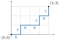
Count the shortest paths from the corner $(0,0)$ to the corner $(4, 3)$ of a grid, moving only one step right (R) or one step up (U) at a time. Every such path takes exactly $7$ steps, of which $4$ are R and $3$ are U; conversely, any word of length $7$ in the letters R, U with four R’s describes exactly one path. The paths therefore correspond bijectively to the choices of the positions of the R’s:

\binom{7}{4} = 35 .

The insight is the encoding: the count became trivial the moment each path was translated into a word, i.e. a subset of positions — one more instance of the slogan that a correct count is a disguised bijection (Method 2.19).

One of the 74 = 35 shortest paths from (0,0) to (4,3): the path shown encodes the word RURRURU, i.e. the choice of positions \1,3,4,6\ for the letter R among the seven steps. — One of the $\binom74 = 35$ shortest paths from $(0,0)$ to $(4,3)$ : the path shown encodes the word RURRURU, i.e. the choice of positions $\{1,3,4,6\}$ for the letter R among the seven steps.

2.3 Lists, permutations, subsets

Definition 2.11 (Arrangements, permutations, combinations)

Let $E$ be a set with $\abs{E} = n$ and let $0 \leq k \leq n$ .

A $k$ -arrangement of $E$ is an injective $k$ -tuple of elements of $E$ (an ordered selection without repetition);
a permutation of $E$ is a bijection from $E$ to itself — equivalently, an $n$ -arrangement;
a $k$ -combination is a subset of $E$ with $k$ elements (an unordered selection without repetition). Their number is written $\binom{n}{k}$ , read “ $n$ choose $k$ ” .

Theorem 2.12 (The three counts)

With $n = \abs{E}$ and $0 \leq k \leq n$ :

the number of $k$ -arrangements of $E$ is $n (n-1) \cdots (n-k+1) = \dfrac{n!}{(n-k)!}$ ;
the number of permutations of $E$ is $n!$ ;
$\dbinom{n}{k} = \dfrac{n!}{k!\,(n-k)!}$ .

Proof. (1) Choose the first coordinate ( $n$ ways), then the second ( $n - 1$ remaining choices), …, then the $k$ -th ( $n - k + 1$ choices). Formally, induct on $k$ . For $k = 1$ there are $n$ one-term injective tuples. Assume the count for $k - 1$ . Each $k$ -arrangement $(x_1, \dots, x_k)$ is obtained from exactly one $(k-1)$ -arrangement — its truncation $(x_1, \dots, x_{k-1})$ — by appending a last coordinate outside $\{x_1, \dots, x_{k-1}\}$ , for which exactly $n - (k - 1)$ values are available. The $k$ -arrangements are thus partitioned, by truncation, into classes of common size $n - k + 1$ indexed by the $(k-1)$ -arrangements, and the sum rule gives

\frac{n!}{(n-k+1)!}\;(n - k + 1) = \frac{n!}{(n-k)!} .

(2) is (1) with $k = n$ .

(3) Each $k$ -subset orders into $k!$ distinct $k$ -arrangements, and every $k$ -arrangement arises from exactly one subset: so $\frac{n!}{(n-k)!} = \binom nk \cdot k!$ . ∎

Example 2.13 (Round tables: quotienting by symmetry)

In how many ways can $n$ guests sit around a round table, two seatings being identical when each guest has the same left and right neighbors — i.e. up to rotation? Each circular seating corresponds to exactly $n$ linear seatings (cut the circle at any of the $n$ places), so the $n!$ linear orders collapse in groups of $n$ :

\frac{n!}{n} = (n-1)! \quad\text{circular seatings.}

Equivalently: seat one distinguished guest anywhere (killing the rotational freedom), then order the remaining $n - 1$ guests clockwise. For $n = 6$ : $120$ tables. The two solutions illustrate the two standard cures for overcounting: divide by the exact number of repetitions, or break the symmetry by pinning one object down. Both require the group-of-repetitions size to be the same for every configuration — which the proof of the formula $\binom nk = \frac{n!}{k!\,(n-k)!}$ above used as well, with $k!$ in place of $n$ .

Example 2.14 (Adding a constraint)

Continuing the round table: among the $(n-1)!$ tables of $n \geq 3$ guests, how many seat two given guests $A$ and $B$ apart (not adjacent)? Count the complement. Tables where $A$ and $B$ sit together: glue them into a single block — $n - 1$ objects around the table, i.e. $(n-2)!$ circular arrangements — then order the pair inside its block ( $2$ ways): $2\,(n-2)!$ adjacent tables. Hence

(n-1)! - 2\,(n-2)! = (n-2)!\,\bigl((n - 1) - 2\bigr) = (n-3)\,(n-2)!

tables keep them apart. Sanity checks: $n = 3$ gives $0$ (around a triangle, everyone touches everyone) and $n = 4$ gives $2$ , easily listed by hand. The gluing trick — treat a forced block as one object, then count its internal arrangements — is the standard cure for adjacency constraints, linear or circular.

Proposition 2.15 (Basic identities)

For $0 \leq k \leq n$ :

\binom{n}{k} = \binom{n}{n-k}, \qquad \binom{n}{k} = \binom{n-1}{k-1} + \binom{n-1}{k} \quad (1 \leq k \leq n-1), \qquad \sum_{k=0}^{n} \binom{n}{k} = 2^n .

Proof. First identity: $A \mapsto E \setminus A$ is a bijection between $k$ -subsets and $(n-k)$ -subsets. Pascal’s rule: fix an element $a \in E$ ; the $k$ -subsets split into those containing $a$ (choose the $k - 1$ others: $\binom{n-1}{k-1}$ ) and those avoiding $a$ ( $\binom{n-1}{k}$ ). Third identity: both sides count all subsets of $E$ , split by size on the left (Proposition 2.8 (1) and (5)). ∎

Theorem 2.16 (Binomial theorem)

For all $a, b$ in a commutative ring (say $\R$ or $\C$ ) and $n \in \N$ :

(a + b)^n = \sum_{k=0}^{n} \binom{n}{k} a^k b^{\,n-k} .

Proof. Expanding $(a+b)(a+b)\cdots(a+b)$ distributively yields one term per choice, in each factor, of either $a$ or $b$ : the term $a^k b^{n-k}$ appears once for each way of choosing which $k$ of the $n$ factors contribute $a$ — that is, $\binom nk$ times. (Alternatively: induct on $n$ using Pascal’s rule.) ∎

Example 2.17

Two classical specializations: $a = b = 1$ recovers $\sum_k \binom nk = 2^n$ ; $a = -1$ , $b = 1$ gives $\sum_{k} (-1)^k \binom nk = 0$ for $n \geq 1$ : among the subsets of a nonempty set, exactly half have even cardinality.

Example 2.18 (One identity, two proofs)

The specialization $a = 2$ , $b = 1$ of the binomial theorem reads

\sum_{k=0}^{n} \binom nk\,2^k = 3^n .

Here is the same identity with no algebra at all. The right side counts the words of length $n$ over the alphabet $\{0, 1, 2\}$ (product rule). Classify each word by the set $K$ of positions carrying a nonzero letter: choosing $K$ with $\abs K = k$ costs $\binom nk$ , then each position of $K$ independently carries $1$ or $2$ : $2^k$ ways. The sum rule over $k$ gives the left side. Beyond the pleasure of agreement, the two proofs have different virtues: the algebraic one generalizes to any value of $a$ , the combinatorial one explains the formula and adapts to constraints (forbid the letter $2$ in the last position, say) that no substitution captures. Keeping both techniques active is the practical skill this chapter trains.

Method 2.19 (Which count applies?)

Before computing, answer two questions about the selection: does the order matter, and are repetitions allowed?

	order matters	order does not matter
no repetition	$\dfrac{n!}{(n-k)!}$	$\dbinom{n}{k}$
[6pt] repetition allowed	$n^k$	(Exercise 2.10)

Then hunt for a bijection or a partition reducing the problem to these model counts; a correct count is a disguised bijection.

Remark 2.20 (Common pitfalls in counting)

Summing non-disjoint cases. The sum rule requires a partition; if configurations can satisfy two cases at once, they are counted twice — the cure is inclusion–exclusion (Theorem 2.24) or a finer case split.
Ordered versus unordered. Choosing “a committee of two” is $\binom n2$ , not $n(n-1)$ : decide before computing whether the selection carries an order, and if an ordered count is easier, divide by the number of orderings at the end — but only when every unordered object arises from the same number of ordered ones.
Multi-stage choices that are not independent. The product rule needs the number of options at each stage to be independent of the previous choices. “Choose a captain, then a different vice-captain” is fine ( $n(n-1)$ ); “choose two players who get along” is not a two-stage product at all.
Double-counting by construction. Building each object twice — e.g. counting hands with at least one ace as (choose an ace) $\times$ (choose $4$ more cards) — overcounts hands with two aces. “At least” almost always calls for the complement (Example 2.9).

Example 2.21 (Poker-style count)

From a $52$ -card deck, the number of $5$ -card hands is $\binom{52}{5} = 2\,598\,960$ . Hands containing exactly one ace: choose the ace ( $4$ ways) then $4$ cards among the $48$ non-aces: $4 \binom{48}{4} = 778\,320$ . The product rule applies because the choice splits into independent stages.

Method 2.22 (Double counting)

To prove an identity between two counting expressions, find a single finite set that both sides count — typically a set of pairs — and evaluate its cardinality in two different orders. The prototype is the handshake lemma: at a party, count the pairs (person, hand shaken). Summing over people gives $\sum_p d_p$ (each person $p$ ’s number of handshakes); summing over handshakes gives twice the number of handshakes (each involves two people). Hence $\sum_p d_p$ is even — so the number of people who shook an odd number of hands is always even, a nontrivial conclusion obtained with no formula at all. The same engine runs Exercise 2.12 and several questions of the weekend problem below.

Example 2.23 (The average subset)

What is the average cardinality of a subset of an $n$ -element set $E$ , all $2^n$ subsets being equally likely? Double count the pairs $(A, a)$ with $a \in A$ : summing over subsets gives $\sum_A \abs A$ , the total we want; summing over elements gives $n \cdot 2^{n-1}$ (each of the $n$ elements lies in exactly half of the subsets — pair each $A$ containing $a$ with $A \setminus \{a\}$ ). Hence

\frac{1}{2^n}\sum_{A \subseteq E} \abs A = \frac{n\,2^{n-1}}{2^n} = \frac n2 :

subsets are, on average, half-full — as the symmetry $A \leftrightarrow \overline A$ (which pairs sizes $k$ and $n - k$ ) also predicts. Two proofs, one answer, and both avoid the direct computation $\sum_k k\binom nk$ of Exercise 2.5: a well-chosen pairing often replaces an identity.

2.4 Inclusion–exclusion

Theorem 2.24 (Inclusion–exclusion)

For finite sets $A_1, \dots, A_p$ :

\Bigl|\, \bigcup_{i=1}^{p} A_i \,\Bigr| = \sum_{\emptyset \neq I \subseteq \intint{1}{p}} (-1)^{\abs{I}+1} \Bigl|\, \bigcap_{i \in I} A_i \,\Bigr| .

For $p = 3$ : $\abs{A \cup B \cup C} = \abs A + \abs B + \abs C - \abs{A \cap B} - \abs{A \cap C} - \abs{B \cap C} + \abs{A \cap B \cap C}$ .

Proof. Fix an element $x$ of the union and count its contribution to the right-hand side. Let $J = \{i : x \in A_i\}$ , of cardinality $m \geq 1$ . The element $x$ is counted once in $\abs{\bigcap_{i \in I} A_i}$ exactly when $\emptyset \neq I \subseteq J$ , with sign $(-1)^{\abs I + 1}$ ; its total contribution is

\sum_{k=1}^{m} \binom{m}{k} (-1)^{k+1} = 1 - \sum_{k=0}^{m} \binom mk (-1)^k = 1 - 0 = 1

by Example 2.17. So each element of the union is counted exactly once. ∎

Example 2.25 (Counting coprime integers)

How many integers of $\intint1{120}$ are coprime to $120 = 2^3 \times 3 \times 5$ ? An integer shares a factor with $120$ exactly when it is divisible by $2$ , $3$ or $5$ , so count the complement of $A_2 \cup A_3 \cup A_5$ , where $A_d$ collects the multiples of $d$ . Within $\intint1{120}$ , the multiples of $d$ number $120/d$ whenever $d$ divides $120$ — no floor functions needed — and $A_2 \cap A_3 = A_6$ , etc. Inclusion–exclusion:

\abs{A_2 \cup A_3 \cup A_5} = 60 + 40 + 24 - 20 - 12 - 8 + 4 = 88 ,

so $120 - 88 = 32$ integers are coprime to $120$ . It is instructive to regroup the computation as a product:

120 - 88 = 120\Bigl(1 - \frac12\Bigr)\Bigl(1 - \frac13\Bigr)\Bigl(1 - \frac15\Bigr) = 120 \cdot \frac12 \cdot \frac23 \cdot \frac45 = 32 :

expanding the three parentheses reproduces exactly the eight signed terms of inclusion–exclusion, one per subset of $\{2, 3, 5\}$ . This product form defines Euler’s totient function, whose arithmetic role appears with Chapter 6’s congruences and is developed in the Year 2 volume.

Example 2.26 (Derangements)

A derangement is a permutation with no fixed point. Let $A_i$ be the set of permutations of $\intint{1}{n}$ fixing $i$ ; then $\abs{\bigcap_{i \in I} A_i} = (n - \abs I)!$ , and inclusion–exclusion counts the permutations with at least one fixed point; the derangements number

D_n = n! \sum_{k=0}^{n} \frac{(-1)^k}{k!} .

Since $\sum (-1)^k / k! \to \eu^{-1}$ (see Chapter 17), about $37\%$ of all permutations are derangements, whatever $n$ is.

Remark 2.27 (Where this chapter is used)

Binomial coefficients are the most heavily reused objects of this chapter: they drive the binomial theorem in Chapter 8 (expansion of $(X + a)^n$ ), the Leibniz formula for the $n$ -th derivative of a product in Chapter 14, and the coefficients of Taylor expansions in Chapter 16. Permutations return as a group — with the signature built from counting inversions — in Chapter 7, and the signature in turn defines determinants in Chapter 22. Inclusion–exclusion and the counting principles are the finite backbone of discrete probability, developed in the Year 2 volume; the derangement numbers of Example 2.26 are studied in depth in the weekend problem below.

2.5 Exercises

Exercise 2.1 ★

A license plate consists of two letters (A–Z), then three digits, then two letters. How many plates are possible? How many with no repeated letter among the four?

Solution

Solution of Exercise 2.1.

Independent stages and the product rule: $26^2 \times 10^3 \times 26^2 = 26^4 \times 1000 = 456\,976\,000$ plates. With the four letters pairwise distinct, the letter stages form a $4$ -arrangement of the alphabet: $26 \times 25 \times 24 \times 23 = 358\,800$ ways, so $358\,800 \times 1000 = 358\,800\,000$ plates.

Exercise 2.2 ★

How many anagrams (rearrangements of the letters, meaningful or not) has the word orange? And banana?

Solution

Solution of Exercise 2.2.

orange has $6$ distinct letters: $6! = 720$ anagrams. banana has $6$ letters with repetitions ( $3$ a’s, $2$ n’s, $1$ b): each anagram is determined by the positions of the a’s ( $\binom 63$ choices), then of the n’s among the remaining $3$ spots ( $\binom 32$ ), the b taking the last spot: $\binom{6}{3}\binom{3}{2} = 20 \times 3 = 60$ anagrams (equivalently $6!/(3!\,2!\,1!) = 60$ ).

Exercise 2.3 ★

A committee of $4$ people is chosen from $7$ women and $5$ men. How many committees: in total? with exactly $2$ women? with at least one man?

Solution

Solution of Exercise 2.3.

Total: $\binom{12}{4} = 495$ . Exactly $2$ women: choose them ( $\binom 72 = 21$ ) and $2$ men ( $\binom 52 = 10$ ): $210$ committees. At least one man: complement of “no man”, $\binom{12}{4} - \binom{7}{4} = 495 - 35 = 460$ .

Exercise 2.4 ★

Prove that in any group of $13$ people, two share their birth month; and that among any $n + 1$ integers chosen from $\intint{1}{2n}$ , two are consecutive. (Pigeonhole both times: name the boxes.)

Solution

Solution of Exercise 2.4.

Birthdays: the boxes are the $12$ months; $13$ people into $12$ boxes force two in the same box (Corollary 2.3).

Consecutive integers: the boxes are the $n$ pairs $\{1,2\}, \{3,4\}, \dots, \{2n-1, 2n\}$ , which partition $\intint{1}{2n}$ . Choosing $n + 1$ integers puts two in the same pair, and the two elements of a pair are consecutive.

Exercise 2.5 ★

Compute $\sum_{k=0}^{n} k \binom{n}{k}$ . Hint: differentiate $(1 + x)^n$ , or use $k \binom nk = n \binom{n-1}{k-1}$ (prove it).

Solution

Solution of Exercise 2.5.

For $1 \leq k \leq n$ ,

k \binom nk = k\,\frac{n!}{k!\,(n-k)!} = n\,\frac{(n-1)!}{(k-1)!\,(n-k)!} = n \binom{n-1}{k-1}.

Summing and reindexing with $j = k - 1$ :

\sum_{k=0}^{n} k \binom nk = n \sum_{j=0}^{n-1} \binom{n-1}{j} = n\, 2^{n-1}

by Proposition 2.15. (Alternative: differentiate $(1+x)^n = \sum_k \binom nk x^k$ and set $x = 1$ .)

Exercise 2.6 ★★

How many strictly increasing maps are there from $\intint{1}{k}$ to $\intint{1}{n}$ ? Deduce the number of increasing (not necessarily strictly) maps. Hint for the second count: $f$ increasing $\mapsto$ $g(i) = f(i) + i - 1$ .

Solution

Solution of Exercise 2.6.

A strictly increasing map $f \colon \intint{1}{k} \to \intint{1}{n}$ is determined by its image, a $k$ -subset of $\intint{1}{n}$ (list the subset in increasing order); conversely every $k$ -subset gives exactly one such map. Hence $\binom nk$ strictly increasing maps.

If $f$ is merely increasing, set $g(i) = f(i) + i - 1$ . Then $g$ is strictly increasing (between consecutive arguments, $f$ gains $\geq 0$ and $i - 1$ gains $1$ ) with values in $\intint{1}{n + k - 1}$ ; and $f(i) = g(i) - i + 1$ recovers $f$ from any strictly increasing $g$ into $\intint{1}{n+k-1}$ . This is a bijection, so there are $\binom{n + k - 1}{k}$ increasing maps.

Exercise 2.7 ★★

(Vandermonde) Prove, by counting $k$ -subsets of a set split into two blocks of sizes $m$ and $n$ :

\binom{m+n}{k} = \sum_{j=0}^{k} \binom{m}{j} \binom{n}{k-j} .

Deduce $\sum_{j=0}^{n} \binom nj^2 = \binom{2n}{n}$ .

Solution

Solution of Exercise 2.7.

Split a set $E$ with $m + n$ elements into blocks $M$ ( $m$ elements) and $N$ ( $n$ elements). A $k$ -subset of $E$ contains some $j$ elements of $M$ ( $0 \leq j \leq k$ ) and $k - j$ of $N$ ; for fixed $j$ there are $\binom mj \binom{n}{k-j}$ such subsets, and the cases $j = 0, \dots, k$ partition the $k$ -subsets. The sum rule gives Vandermonde’s identity.

With $m = n = k$ : $\binom{2n}{n} = \sum_{j=0}^{n} \binom nj \binom{n}{n-j} = \sum_{j=0}^{n} \binom nj^2$ , using $\binom{n}{n-j} = \binom nj$ .

Exercise 2.8 ★★

How many integers in $\intint{1}{1000}$ are divisible by $2$ or $3$ or $5$ ? (Inclusion–exclusion; $\lfloor 1000/6 \rfloor$ counts the multiples of $6$ , etc.)

Solution

Solution of Exercise 2.8.

Let $A_d$ be the multiples of $d$ in $\intint{1}{1000}$ , so $\abs{A_d} = \lfloor 1000/d \rfloor$ . Inclusion–exclusion (Theorem 2.24) with $A_2, A_3, A_5$ , noting $A_2 \cap A_3 = A_6$ etc.:

500 + 333 + 200 - 166 - 100 - 66 + 33 = 734 .

So $734$ integers are divisible by $2$ , $3$ or $5$ .

Exercise 2.9 ★★

Count the surjections from a set of $4$ elements onto a set of $2$ elements; then onto a set of $3$ elements. Hint: count the non-surjective maps with inclusion–exclusion on the missed values.

Solution

Solution of Exercise 2.9.

Onto $2$ elements: all $2^4 = 16$ maps except the $2$ constant maps: $14$ surjections.

Onto $3$ elements: by inclusion–exclusion on the missed values, the number of maps from a $4$ -set to a $3$ -set missing at least one value is $\binom 31 2^4 - \binom 32 1^4 = 48 - 3 = 45$ ; total maps $3^4 = 81$ ; surjections: $81 - 45 = 36$ . (Check: a surjection from $4$ onto $3$ elements doubles up exactly one value: choose the doubled value ( $3$ ), the pair mapping to it ( $\binom 42 = 6$ ), and a bijection for the rest ( $2$ ): $3 \times 6 \times 2 = 36$ .)

Exercise 2.10 ★★

(Stars and bars) Prove that the number of $k$ -selections of $n$ objects with repetition, order ignored — equivalently, the number of $(x_1, \dots, x_n) \in \N^n$ with $x_1 + \dots + x_n = k$ — is $\binom{n + k - 1}{k}$ . Hint: encode a solution as a row of $k$ stars and $n - 1$ bars.

Solution

Solution of Exercise 2.10.

A solution of $x_1 + \dots + x_n = k$ in $\N^n$ encodes as a row of $k$ stars and $n - 1$ bars: write $x_1$ stars, a bar, $x_2$ stars, a bar, …, ending with $x_n$ stars. This is a bijection onto the words of length $k + n - 1$ using $k$ stars and $n - 1$ bars, and those words are determined by the positions of the stars: $\binom{n + k - 1}{k}$ . Selections with repetition correspond to solutions of the equation ( $x_i$ = number of copies of object $i$ ), so the count is the same.

Exercise 2.11 ★★★

Prove the formula of Example 2.26 for $D_n$ in detail, and deduce $n! = \sum_{k=0}^{n} \binom{n}{k} D_{n-k}$ (also prove this identity directly by classifying permutations by their fixed-point set).

Solution

Solution of Exercise 2.11.

With $A_i = \{\sigma : \sigma(i) = i\}$ , a permutation in $\bigcap_{i \in I} A_i$ fixes every $i \in I$ and permutes the other $n - \abs I$ points freely: $\abs{\bigcap_{i \in I} A_i} = (n - \abs I)!$ . Inclusion–exclusion:

\Bigl|\bigcup_i A_i\Bigr| = \sum_{k=1}^{n} (-1)^{k+1} \binom nk (n-k)! = \sum_{k=1}^{n} (-1)^{k+1} \frac{n!}{k!} ,

since there are $\binom nk$ subsets $I$ of size $k$ . Hence

D_n = n! - \Bigl|\bigcup_i A_i\Bigr| = n!\Bigl(1 - \sum_{k=1}^{n} \frac{(-1)^{k+1}}{k!}\Bigr) = n! \sum_{k=0}^{n} \frac{(-1)^k}{k!} .

For the second identity: classify the permutations $\sigma$ of $\intint{1}{n}$ by their fixed-point set $F(\sigma)$ . For a fixed $k$ -subset $F$ , the permutations with $F(\sigma) = F$ are exactly the derangements of the complement: $D_{n-k}$ of them. Summing over the $\binom nk$ choices of $F$ for each $k$ : $n! = \sum_{k=0}^{n} \binom nk D_{n-k}$ .

Exercise 2.12 ★★★

For $n \in \N^*$ , prove by a double count of pairs (subset, marked element):

\sum_{k=1}^{n} k \binom{n}{k} = n\, 2^{n-1}, \qquad\text{then}\qquad \sum_{k=1}^{n} k^2 \binom{n}{k} = n(n+1)\, 2^{n-2} .

For the second: count pairs of marked elements, equal or not.

Solution

Solution of Exercise 2.12.

First identity. Count the pairs $(A, a)$ where $A \subseteq E$ ( $\abs E = n$ ) and $a \in A$ . By size of $A$ : $\sum_k \binom nk k$ pairs. By choosing the marked element first: $n$ choices for $a$ , then any subset of the remaining $n - 1$ elements to complete $A$ : $n\,2^{n-1}$ pairs.

Second identity. Count the triples $(A, a, b)$ with $a, b \in A$ (possibly $a = b$ ). By size: $\sum_k k^2 \binom nk$ . Directly: either $a = b$ ( $n\,2^{n-1}$ triples, previous count) or $a \neq b$ ( $n(n-1)$ ordered choices, then any subset of the other $n - 2$ elements: $n(n-1)\,2^{n-2}$ ). Total

n\,2^{n-1} + n(n-1)\,2^{n-2} = n\,2^{n-2}\,(2 + n - 1) = n(n+1)\,2^{n-2} .

2.6 Problem: Derangements, or the misaddressed letters

Problem 2.1

A secretary puts $n$ letters into $n$ addressed envelopes at random: what is the chance that nobody receives the right letter? This classical question (Montmort, 1708) leads to the derangement numbers $D_n$ of Example 2.26. The inclusion–exclusion formula is only the opening move: this problem develops the recurrences that compute $D_n$ , two further independent proofs of the formula, the striking theorem that $D_n$ is the integer nearest to $n!/\eu$ , the full distribution of fixed points of a random permutation, and the curious arithmetic of the sequence $(D_n)$ . Throughout, $D_n$ denotes the number of derangements (fixed-point free permutations) of $\intint1n$ , with the convention $D_0 = 1$ (the empty permutation has no fixed point).

Part I — Small cases and the fixed-point census.

Compute $D_1, D_2, D_3$ directly, and $D_4$ by listing the derangements of $\{1, 2, 3, 4\}$ grouped by the value of $\sigma(1)$ . (You should find $D_4 = 9$ .)
For $0 \leq k \leq n$ , show that the number $P_k(n)$ of permutations of $\intint1n$ with exactly $k$ fixed points is $\binom nk D_{n-k}$ .
Verify the census for $n = 4$ : compute $P_0(4), \dots, P_4(4)$ and check that they sum to $4! = 24$ . Which is more likely for four letters: no match, or exactly one match?
By double counting (Method 2.22) the pairs $(\sigma, i)$ with $\sigma(i) = i$ , show that

$\sum_{\sigma} \abs{\mathrm{Fix}(\sigma)} = n! :$

on average, a random permutation has exactly one fixed point, whatever $n \geq 1$ is.

Part II — Two recurrences and two new proofs of the formula.

Prove combinatorially, for $n \geq 1$ :

$D_{n+1} = n\,(D_n + D_{n-1}) .$

(Classify the derangements $\sigma$ of $\intint1{n+1}$ by $j = \sigma(n+1)$ , then by whether $\sigma(j) = n + 1$ ; in the case $\sigma(j) \neq n+1$ , build a bijection with the derangements of $\intint1n$ by redirecting the preimage of $n + 1$ to $j$ .) Check the recurrence numerically up to $D_6$ .
Setting $u_n = D_n - n D_{n-1}$ , deduce from question 5 that $u_{n+1} = -u_n$ , and conclude the second recurrence:

$D_n = n D_{n-1} + (-1)^n \qquad (n \geq 1).$
From question 6, prove by induction the formula of Example 2.26,

$D_n = n! \sum_{k=0}^{n} \frac{(-1)^k}{k!},$

— a proof wholly independent of inclusion–exclusion.
(Binomial inversion) Let $(a_n)$ and $(b_n)$ be two sequences such that $a_n = \sum_{k=0}^n \binom nk b_k$ for all $n$ . Prove that

$b_n = \sum_{k=0}^{n} (-1)^{n-k} \binom nk a_k \qquad (n \in \N).$

(First establish the trinomial revision $\binom nk \binom kj = \binom nj \binom{n-j}{k-j}$ , then use the alternating row sum of Example 2.17.)
Apply question 8 to the identity $n! = \sum_k \binom nk D_{n-k}$ of Exercise 2.11 to obtain a third proof of the formula for $D_n$ .

Part III — The nearest integer to $n!/\eu$ . Admit for this part — the theory is built in Chapter 17 — that $\eu^{-1} = \lim_{n \to \infty} s_n$ where $s_n = \sum_{k=0}^{n} \frac{(-1)^k}{k!}$ , with the strict alternating-series bound $\abs{\eu^{-1} - s_n} < \frac1{(n+1)!}$ for every $n$ .

Show that $\bigl| D_n - n!/\eu \bigr| < \frac1{n+1}$ for all $n \in \N$ .
Deduce the headline theorem: for every $n \geq 1$ , $D_n$ is the integer nearest to $n!/\eu$ . Why does the argument need $n \geq 1$ ?
Determine the sign of the error: show that $D_n > n!/\eu$ exactly when $n$ is even. (Locate the first neglected term of the alternating series.)
Compute $D_7$ through $D_{10}$ with the recurrence of question 5, then check $D_{10}$ against $10!/\eu$ ( $10! = 3\,628\,800$ , $\eu \approx 2.718281828$ ).
(The hat-check probability) Let $p_n = D_n/n!$ be the probability that a uniformly random permutation is a derangement. Show $\abs{p_n - \eu^{-1}} < \frac1{(n+1)!}$ and compute $p_6$ to five decimal places. Comment: why is the answer to Montmort’s question essentially independent of $n$ — already for a dozen letters?

Part IV — The distribution of fixed points.

Fix $k \in \N$ . Show that the proportion of permutations of $\intint1n$ with exactly $k$ fixed points satisfies

$\frac{P_k(n)}{n!} = \frac{s_{n-k}}{k!} \;\xrightarrow[n \to \infty]{}\; \frac{\eu^{-1}}{k!} .$

(These limiting values, summing to $1$ , form the Poisson distribution of parameter $1$ , a central object of the probability course in the Year 2 volume.)
By double counting the triples $(\sigma, i, j)$ where $i \neq j$ are both fixed by $\sigma$ , show that $\sum_\sigma \abs{\mathrm{Fix}(\sigma)}\, (\abs{\mathrm{Fix}(\sigma)} - 1) = n!$ for $n \geq 2$ . Combined with question 4: the average of $\abs{\mathrm{Fix}}^2$ is $2$ , so the “spread” (variance) of the number of fixed points equals $1$ — again independent of $n$ , again matching the Poisson law.
Compute the proportion of permutations having at least one fixed point for $n = 4, 5, 6$ (as fractions and to four decimal places), and compare with $1 - \eu^{-1} \approx 0.6321$ .
Show directly — no limits needed — that $s_{n+2} - s_n = (-1)^{n+1}\bigl(\frac1{(n+1)!} - \frac1{(n+2)!}\bigr)$ , and deduce that the probabilities $p_n = s_n$ of question 14 oscillate: $p_0 > p_2 > p_4 > \dots$ and $p_1 < p_3 < p_5 < \dots$ , the even (resp. odd) values decreasing (resp. increasing) toward the common limit $\eu^{-1}$ .
(Secret Santa) $n$ people each draw one name from a hat; if anyone draws their own name, the whole drawing is restarted from scratch. Using the standard fact that an event of probability $p$ takes on average $1/p$ attempts, estimate the average number of complete drawings needed, and conclude that the procedure costs about $\eu \approx 2.72$ drawings on average, essentially independently of $n$ .

Part V — The arithmetic of $D_n$ , and a synthesis.

Refine question 5: show that for fixed $j \in \intint2n$ , the derangements of $\intint1n$ with $\sigma(1) = j$ number exactly $D_{n-1} + D_{n-2}$ , independently of $j$ . Deduce that $n - 1$ divides $D_n$ for every $n \geq 2$ .
Prove that $D_n$ is odd if and only if $n$ is even. (Work modulo $2$ in the recurrence of question 6.)
Prove that $D_n \equiv (-1)^n \pmod n$ for $n \geq 1$ , and check the congruence on the last digit of $D_{10}$ .
Show from question 6 that $\dfrac{D_n}{D_{n-1}} = n + \dfrac{(-1)^n}{D_{n-1}}$ for $n \geq 3$ , so the ratio of consecutive derangement numbers is almost exactly $n$ ; explain in one sentence why this is consistent with $D_n \approx n!/\eu$ .
Where exactly did this problem use: (i) the product and sum rules; (ii) double counting; (iii) the binomial theorem; (iv) the admitted alternating-series bound? One sentence each.
Synthesis. The formula for $D_n$ now has three proofs (inclusion–exclusion, recurrence plus induction, binomial inversion). In a short paragraph, compare what each proof explains: which one computes fastest, which one generalizes to other fixed-point counts, and which one reveals why $\eu$ appears in a problem about envelopes.

Solution

Solution of Problem 2.1.

1. $D_1 = 0$ (the only permutation fixes $1$ ), $D_2 = 1$ (the swap), $D_3 = 2$ (in one-line notation: $231$ and $312$ ). For $n = 4$ , group by $\sigma(1)$ : with $\sigma(1) = 2$ the derangements are $2143$ , $2341$ , $2413$ ; with $\sigma(1) = 3$ : $3142$ , $3412$ , $3421$ ; with $\sigma(1) = 4$ : $4123$ , $4312$ , $4321$ . Three in each group: $D_4 = 9$ .

2. A permutation with exactly $k$ fixed points is determined by the choice of its fixed-point set $F$ ( $\binom nk$ ways) together with its restriction to the complement, which must be a permutation of $n - k$ points with no fixed point ( $D_{n-k}$ ways). The two choices are independent and the correspondence is bijective: $P_k(n) = \binom nk D_{n-k}$ .

3. $P_0(4) = D_4 = 9$ ; $P_1(4) = \binom41 D_3 = 4 \times 2 = 8$ ; $P_2(4) = \binom42 D_2 = 6$ ; $P_3(4) = \binom43 D_1 = 0$ (three fixed points force a fourth); $P_4(4) = 1$ . Sum: $9 + 8 + 6 + 0 + 1 = 24 = 4!$ . No match ( $9$ cases) beats exactly one match ( $8$ cases) — narrowly.

4. Count the pairs $(\sigma, i)$ with $\sigma(i) = i$ . For fixed $i$ , the permutations fixing $i$ are the permutations of the other $n - 1$ points: $(n-1)!$ of them. Hence the number of pairs is $n \cdot (n-1)! = n!$ , and this number is also $\sum_\sigma \abs{\mathrm{Fix}(\sigma)}$ . Dividing by the number $n!$ of permutations: the average number of fixed points is exactly $1$ , for every $n \geq 1$ .

5. Let $\sigma$ be a derangement of $\intint1{n+1}$ and $j = \sigma(n+1) \in \intint1n$ : $n$ possible values. Case $\sigma(j) = n+1$ : the points $j$ and $n+1$ swap, and $\sigma$ restricted to the remaining $n - 1$ points is an arbitrary derangement of them: $D_{n-1}$ possibilities. Case $\sigma(j) \neq n+1$ : let $i_0 = \sigma^{-1}(n+1)$ ; here $i_0 \neq j$ and $i_0 \leq n$ . Define $\tau$ on $\intint1n$ by $\tau(i) = \sigma(i)$ for $i \neq i_0$ and $\tau(i_0) = j$ . Then $\tau$ is a permutation of $\intint1n$ (the value $n+1$ has been replaced by the missing value $j$ ), and it is a derangement: $\tau(i_0) = j \neq i_0$ , and $\tau(i) = \sigma(i) \neq i$ elsewhere. Conversely, from a derangement $\tau$ of $\intint1n$ and the value $j$ , one recovers $\sigma$ by setting $\sigma(n+1) = j$ , $\sigma(\tau^{-1}(j)) = n+1$ and $\sigma = \tau$ elsewhere: a bijection, giving $D_n$ possibilities. Summing over $j$ : $D_{n+1} = n(D_n + D_{n-1})$ . Numerically: $D_5 = 4(9 + 2) = 44$ , $D_6 = 5(44 + 9) = 265$ .

6. From question 5, $D_{n+1} = nD_n + nD_{n-1}$ , so

u_{n+1} = D_{n+1} - (n+1)D_n = nD_n + nD_{n-1} - (n+1)D_n = -(D_n - nD_{n-1}) = -u_n .

Since $u_1 = D_1 - 1 \cdot D_0 = -1$ , induction gives $u_n = (-1)^n$ , i.e. $D_n = nD_{n-1} + (-1)^n$ for $n \geq 1$ .

7. Induction on $n$ . Base: $D_0 = 1 = 0!\,s_0$ . Step: assuming $D_{n-1} = (n-1)!\,s_{n-1}$ ,

D_n = nD_{n-1} + (-1)^n = n!\,s_{n-1} + (-1)^n = n!\Bigl(s_{n-1} + \frac{(-1)^n}{n!}\Bigr) = n!\,s_n ,

which is the formula. No inclusion–exclusion was used: only the combinatorial recurrence of question 5.

8. Trinomial revision, by factorials:

\binom nk \binom kj = \frac{n!}{k!\,(n-k)!} \cdot \frac{k!}{j!\,(k-j)!} = \frac{n!}{j!\,(n-j)!} \cdot \frac{(n-j)!}{(k-j)!\,(n-k)!} = \binom nj \binom{n-j}{k-j} .

Now substitute $a_k = \sum_j \binom kj b_j$ and exchange the two finite sums:

\sum_{k=0}^{n} (-1)^{n-k} \binom nk a_k = \sum_{j=0}^{n} b_j \binom nj \sum_{k=j}^{n} (-1)^{n-k} \binom{n-j}{k-j} = \sum_{j=0}^{n} b_j \binom nj \sum_{i=0}^{n-j} (-1)^{(n-j)-i} \binom{n-j}{i} .

The inner sum is the expansion of $(1 + (-1))^{n-j} = 0^{n-j}$ (binomial theorem, Theorem 2.16): it vanishes for $j < n$ and equals $1$ for $j = n$ . Only $j = n$ survives, and the right-hand side is $b_n$ , as claimed.

9. By the symmetry $\binom nk = \binom n{n-k}$ , the identity of Exercise 2.11 rewrites as $n! = \sum_{k=0}^n \binom nk D_k$ . Apply question 8 with $a_n = n!$ and $b_k = D_k$ :

D_n = \sum_{k=0}^{n} (-1)^{n-k} \binom nk k! = \sum_{k=0}^{n} (-1)^{n-k} \frac{n!}{(n-k)!} = n! \sum_{j=0}^{n} \frac{(-1)^j}{j!} ,

reindexing by $j = n - k$ : the formula a third time.

10. $D_n = n!\,s_n$ (question 7), so

\Bigl| D_n - \frac{n!}{\eu} \Bigr| = n!\,\abs{s_n - \eu^{-1}} < \frac{n!}{(n+1)!} = \frac1{n+1} .

11. For $n \geq 1$ , $\frac1{n+1} \leq \frac12$ , and the inequality of question 10 is strict: $D_n$ lies at distance $< \frac12$ from $n!/\eu$ , so it is the unique nearest integer. For $n = 0$ the bound only gives distance $< 1$ , and indeed the claim fails there: $0!/\eu \approx 0.368$ has nearest integer $0$ , while $D_0 = 1$ .

12. $\eu^{-1} - s_n = \sum_{k \geq n+1} (-1)^k/k!$ is an alternating series with strictly decreasing terms, so its sign is the sign of its first term $(-1)^{n+1}/(n+1)!$ . Hence $s_n - \eu^{-1}$ has the sign of $(-1)^n$ : for $n$ even, $s_n > \eu^{-1}$ and $D_n = n!\,s_n > n!/\eu$ ; for $n$ odd, $D_n < n!/\eu$ .

13. $D_7 = 6(265 + 44) = 6 \times 309 = 1854$ ; $D_8 = 7(1854 + 265) = 7 \times 2119 = 14\,833$ ; $D_9 = 8(14\,833 + 1854) = 8 \times 16\,687 = 133\,496$ ; $D_{10} = 9(133\,496 + 14\,833) = 9 \times 148\,329 = 1\,334\,961$ . Check: $10!/\eu = 3\,628\,800 / 2.718281828 \approx 1\,334\,960.92$ , whose nearest integer is $1\,334\,961$ — and $D_{10} > 10!/\eu$ , as question 12 predicts for even $n$ .

14. $\abs{p_n - \eu^{-1}} = \abs{s_n - \eu^{-1}} < \frac1{(n+1)!}$ . For $n = 6$ : $p_6 = 265/720 = 0.36806$ (five decimals), against $\eu^{-1} = 0.36788$ ; the gap is below $1/7! = 1/5040 < 2 \times 10^{-4}$ . The bound $1/(n+1)!$ collapses so fast that the probability is fixed to many decimal places already for a dozen letters: the answer “about $36.8\%$ ” is, for every practical purpose, independent of $n$ — the famous surprise of the problem.

15. By question 2 and $D_m = m!\,s_m$ :

\frac{P_k(n)}{n!} = \frac{\binom nk D_{n-k}}{n!} = \frac{D_{n-k}}{k!\,(n-k)!} = \frac{s_{n-k}}{k!} \;\longrightarrow\; \frac{\eu^{-1}}{k!}

as $n \to \infty$ with $k$ fixed, since $s_{n-k} \to \eu^{-1}$ . The limit values $\eu^{-1}/k!$ ( $k \in \N$ ) are the weights of the Poisson distribution of parameter $1$ .

16. Count the triples $(\sigma, i, j)$ with $i \neq j$ , $\sigma(i) = i$ , $\sigma(j) = j$ . Choosing the ordered pair first: $n(n-1)$ ways; the permutations fixing both $i$ and $j$ are the permutations of the remaining $n - 2$ points: $(n-2)!$ of them. Total: $n(n-1)(n-2)! = n!$ . Summing instead over $\sigma$ first counts, for each $\sigma$ , the ordered pairs of distinct fixed points: $\abs{\mathrm{Fix}(\sigma)}(\abs{\mathrm{Fix}(\sigma)}-1)$ . Hence the stated identity; dividing by $n!$ , the average of $\abs{\mathrm{Fix}}(\abs{\mathrm{Fix}} - 1)$ is $1$ , so the average of $\abs{\mathrm{Fix}}^2$ is $1 + 1 = 2$ and the variance is $2 - 1^2 = 1$ .

17. The proportions $1 - p_n$ : for $n = 4$ , $1 - \frac 9{24} = \frac{15}{24} = 0.6250$ ; for $n = 5$ , $1 - \frac{44}{120} = \frac{76}{120} = 0.6333$ ; for $n = 6$ , $1 - \frac{265}{720} = \frac{455}{720} = 0.6319$ . All within a percent of $1 - \eu^{-1} \approx 0.6321$ , oscillating around it.

18. Directly:

s_{n+2} - s_n = \frac{(-1)^{n+1}}{(n+1)!} + \frac{(-1)^{n+2}}{(n+2)!} = (-1)^{n+1}\Bigl(\frac1{(n+1)!} - \frac1{(n+2)!}\Bigr),

and the parenthesis is $> 0$ . For $n$ even the difference is negative: $s_{n+2} < s_n$ , so $p_0 > p_2 > p_4 > \dots$ ; for $n$ odd it is positive: $p_1 < p_3 < p_5 < \dots$ Combined with question 12 (evens above $\eu^{-1}$ , odds below) and question 14 (distance to $\eu^{-1}$ tends to $0$ ): the two staircases squeeze $\eu^{-1}$ between them.

19. One complete drawing is a uniform random permutation, valid when it is a derangement: probability $p_n \approx \eu^{-1}$ . By the quoted fact, the average number of drawings until success is $1/p_n$ , and question 14 gives $1/p_n \approx \eu$ up to an error that is negligible already for small $n$ . So a Secret Santa with restarts costs on average about $\eu \approx 2.72$ complete drawings — whether the office has $6$ people or $600$ .

20. Fix $j \geq 2$ and run question 5’s classification on the value $\sigma(1) = j$ . If $\sigma(j) = 1$ : the remaining $n - 2$ points carry an arbitrary derangement, $D_{n-2}$ ways. If $\sigma(j) \neq 1$ : redirect the preimage $i_0 = \sigma^{-1}(1)$ to $j$ exactly as in question 5; this is a bijection with the derangements of the $n - 1$ points $\{2, \dots, n\}$ : $D_{n-1}$ ways. Total $D_{n-1} + D_{n-2}$ , the same for every $j$ . Summing over the $n - 1$ values of $j$ : $D_n = (n-1)(D_{n-1} + D_{n-2})$ , which displays the factor $n - 1$ : $(n-1) \mid D_n$ .

21. Claim: $D_n$ is odd iff $n$ is even. Induction using $D_n = nD_{n-1} + (-1)^n$ , i.e. $D_n \equiv nD_{n-1} + 1 \pmod 2$ . Base: $D_1 = 0$ is even, $n = 1$ odd: claim holds. If $n$ is even, $nD_{n-1}$ is even and $D_n \equiv 1$ : odd, as claimed. If $n$ is odd, then $n - 1$ is even, so $D_{n-1}$ is odd by hypothesis, and $D_n \equiv D_{n-1} + 1 \equiv 0$ : even. The induction closes.

22. Reducing $D_n = nD_{n-1} + (-1)^n$ modulo $n$ kills the first term: $D_n \equiv (-1)^n \pmod n$ . For $n = 10$ : $(-1)^{10} = 1$ , and indeed $D_{10} = 1\,334\,961$ ends in the digit $1$ .

23. For $n \geq 3$ , $D_{n-1} \geq 1$ and division of question 6’s recurrence by $D_{n-1}$ gives $D_n/D_{n-1} = n + (-1)^n/D_{n-1}$ , with $\abs{(-1)^n/D_{n-1}} \leq 1$ and rapidly tending to $0$ . Consistency: if $D_n \approx n!/\eu$ , then $D_n/D_{n-1} \approx n!/(n-1)! = n$ — the factor $\eu$ cancels in the ratio, and the recurrence confirms it to accuracy $1/D_{n-1}$ .

24. (i) The product and sum rules underlie every count: questions 2 and 5 partition sets of permutations into independent stages. (ii) Double counting gave the mean (question 4) and the variance (question 16) of the number of fixed points with no formula for $D_n$ at all. (iii) The binomial theorem evaluated the alternating inner sum $(1-1)^{n-j}$ that makes binomial inversion work (question 8). (iv) The alternating-series bound converted the exact but opaque sum $n!\,s_n$ into the transparent statement “nearest integer to $n!/\eu$ ” (questions 10–14).

25. Inclusion–exclusion (Example 2.26 and Exercise 2.11) is the conceptual proof: it explains the alternating sum as overcounting corrections, and it generalizes verbatim to counting elements avoiding any family of “bad” sets. The recurrence route (questions 5–7) computes fastest — linear time, exact integer arithmetic, no factorials — and is the source of the arithmetic facts of Part V. Binomial inversion (questions 8–9) places the formula inside a general transform that will reappear wherever two triangular systems of identities face each other. And the appearance of $\eu$ is best explained by the formula itself: the proportion of derangements is the partial sum $s_n$ of the series for $\eu^{-1}$ , so Montmort’s envelopes were, three decades before Euler’s notation, already computing the number $\eu$ .