University Mathematics — Year 1 · Bachelor Year 1

8Polynomials

Polynomials are the algebraist’s favorite functions — except that they are not treated as functions here, but as formal expressions in an indeterminate $X$ , added and multiplied by the rules of a commutative ring. The theory runs strikingly parallel to Chapter 6: a Euclidean division, a gcd and Bézout relations, irreducible elements and a unique factorization. Throughout, $K$ denotes $\Q$ , $\R$ or $\C$ .

8.1 The ring $K[X]$

Definition 8.1 (Polynomial, degree)

A polynomial with coefficients in $K$ is a formal sum

P = a_0 + a_1 X + a_2 X^2 + \dots + a_n X^n = \sum_{k} a_k X^k,

with $a_k \in K$ all zero from some index on. With the natural addition and the product

\Bigl(\sum_i a_i X^i\Bigr)\Bigl(\sum_j b_j X^j\Bigr) = \sum_k \Bigl(\sum_{i+j=k} a_i b_j\Bigr) X^k,

the set $K[X]$ is a commutative ring. The degree $\deg P$ of $P \neq 0$ is the largest $n$ with $a_n \neq 0$ ; $a_n$ is the leading coefficient ( $P$ is monic when $a_n = 1$ ), and by convention $\deg 0 = -\infty$ . Every polynomial defines a function $x \mapsto P(x)$ on $K$ by substitution.

Proposition 8.2 (Degree rules; integral domain)

For $P, Q \in K[X]$ :

\deg(P + Q) \leq \max(\deg P, \deg Q), \qquad \deg(PQ) = \deg P + \deg Q .

Consequently $K[X]$ is an integral domain, and its units are the nonzero constants.

Proof. The sum rule is clear (coefficients beyond the max vanish). For the product, let $a_m$ and $b_n$ be the leading coefficients: the coefficient of $X^{m+n}$ in $PQ$ is $a_m b_n \neq 0$ ( $K$ is a field, hence an integral domain), and all higher coefficients vanish. If $P, Q \neq 0$ then $\deg PQ = \deg P + \deg Q \geq 0$ , so $PQ \neq 0$ : integral domain. If $PQ = 1$ then $\deg P + \deg Q = 0$ forces $\deg P = \deg Q = 0$ : invertible elements are the invertible constants, i.e. all of $K^*$ . ∎

Theorem 8.3 (Euclidean division)

Let $A, B \in K[X]$ with $B \neq 0$ . There is exactly one pair $(Q, R)$ of polynomials with

A = BQ + R, \qquad \deg R < \deg B .

Proof. Existence, by strong induction on $\deg A$ . If $\deg A < \deg B$ , take $(Q, R) = (0, A)$ . Otherwise write $A = a X^m + \dots$ , $B = b X^n + \dots$ with $m \geq n$ ; the polynomial $A_1 = A - \frac ab X^{m-n} B$ has degree $< m$ (the leading terms cancel), so by induction $A_1 = BQ_1 + R$ with $\deg R < \deg B$ , and $A = B(Q_1 + \frac ab X^{m-n}) + R$ .

Uniqueness: if $BQ + R = BQ' + R'$ , then $B(Q - Q') = R' - R$ with $\deg(R' - R) < \deg B$ ; by the degree rule this forces $Q - Q' = 0$ , then $R = R'$ . ∎

Example 8.4

Divide $A = X^4 + X^3 - 2X + 1$ by $B = X^2 + 1$ :

X^4 + X^3 - 2X + 1 = (X^2 + 1)(X^2 + X - 1) + (-3X + 2).

(Compute: subtract $X^2 B$ , then $X B$ , then $-B$ ; the remainder $-3X + 2$ has degree $1 < 2$ .)

Method 8.5 (Horner’s scheme)

To evaluate $P = a_nX^n + \dots + a_0$ at $x$ , or to divide $P$ by $X - x$ , avoid computing powers: read the coefficients left to right, and iterate multiply by $x$ , add the next coefficient:

b_n = a_n, \qquad b_{k} = a_{k} + x\,b_{k+1} \quad (k = n-1, \dots, 0) .

Then $b_0 = P(x)$ , and the earlier $b_k$ are the quotient’s coefficients: $P = (X - x)(b_nX^{n-1} + \dots + b_1) + b_0$ (expand and compare). Example: $P = X^4 - 5X^3 + 6X^2 + 4X - 8$ at $x = 2$ : the $b$ ’s are $1, -3, 0, 4, 0$ , so $P(2) = 0$ and $P = (X-2)(X^3 - 3X^2 + 4)$ — one line instead of a long division, and $n$ multiplications instead of the $\approx n^2/2$ of the naive evaluation. Iterating the scheme at the same point extracts multiplicities (compare Example 8.12).

Remark 8.6 (Arithmetic of $K[X]$ )

With Euclidean division in hand, the entire arithmetic of Chapter 6 transfers to $K[X]$ , with the same proofs, degree playing the role of absolute value: gcd (normalized to be monic), extended Euclidean algorithm, Bézout’s identity, Gauss’s lemma, irreducible polynomials and unique factorization. We freely use these transferred results, and Exercise 8.6 rehearses one of them.

8.2 Roots

Theorem 8.7 (Factor theorem)

Let $P \in K[X]$ and $a \in K$ . The remainder of $P$ upon division by $X - a$ is the constant $P(a)$ . In particular

P(a) = 0 \iff (X - a) \mid P .

More generally, distinct roots $a_1, \dots, a_r$ of $P$ give the factorization $P = (X - a_1)\cdots(X - a_r)\, Q$ .

Proof. Divide: $P = (X - a) Q + R$ with $\deg R < 1$ , so $R$ is a constant $c$ ; substituting $X = a$ (substitution respects sums and products) gives $P(a) = c$ . The equivalence follows. For several roots, induct on $r$ : the case $r = 1$ is the equivalence just proved. Assume the statement for $r - 1$ roots and let $a_1, \dots, a_r$ be distinct roots of $P$ . Write $P = (X - a_1)Q_1$ ; for each $i \geq 2$ , substituting $a_i$ :

0 = P(a_i) = (a_i - a_1)\,Q_1(a_i), \qquad a_i - a_1 \neq 0 ,

and since $K$ has no zero divisors, $Q_1(a_i) = 0$ : the $r - 1$ distinct points $a_2, \dots, a_r$ are roots of $Q_1$ . The induction hypothesis factors $Q_1 = (X - a_2)\cdots(X - a_r)\,Q$ , and substituting back gives the claim. ∎

Corollary 8.8 (A polynomial of degree $n$ has at most $n$ roots)

A nonzero $P \in K[X]$ of degree $n$ has at most $n$ distinct roots in $K$ . Consequently, a polynomial (of degree $\leq n$ ) vanishing at $n + 1$ distinct points is the zero polynomial, and two polynomials of degree $\leq n$ agreeing at $n+1$ points are equal.

Proof. If $a_1, \dots, a_r$ are distinct roots, Theorem 8.7 gives $P = (X-a_1)\cdots(X-a_r) Q$ , so $n = \deg P \geq r$ . The two consequences follow by contradiction and by difference. ∎

Example 8.9 (The auxiliary-polynomial trick)

Let $P$ be the polynomial of degree $\leq n$ with

P(k) = \frac{k}{k+1} \qquad (k = 0, 1, \dots, n) ;

it exists and is unique by Lagrange interpolation below. What is $P(n+1)$ ? Clear denominators: the polynomial $Q = (X+1)P - X$ has degree $\leq n + 1$ and vanishes at the $n + 1$ points $0, 1, \dots, n$ , so by Theorem 8.7

Q = c\,X(X-1)(X-2)\cdots(X-n)

for some constant $c$ . Evaluate where $Q$ is known independently: at $X = -1$ , $Q(-1) = 0 \cdot P(-1) + 1 = 1$ , while the product equals $(-1)(-2)\cdots(-1-n) = (-1)^{n+1}(n+1)!$ ; hence $c = \frac{(-1)^{n+1}}{(n+1)!}$ . Now evaluate at $X = n + 1$ :

(n+2)\,P(n+1) - (n+1) = Q(n+1) = c\,(n+1)! = (-1)^{n+1} ,

so $P(n+1) = \dfrac{(n+1) + (-1)^{n+1}}{n+2}$ : equal to $1$ for odd $n$ , and to $\frac{n}{n+2}$ for even $n$ — the interpolating polynomial does not continue the pattern $\frac{n+1}{n+2}$ . The trick to remember: encode the data as roots of an auxiliary polynomial, identify the unknown constant at a point outside the data, and harvest.

Definition 8.10 (Derivative, multiplicity)

The formal derivative of $P = \sum a_k X^k$ is $P' = \sum_{k \geq 1} k\,a_k X^{k-1}$ ; it satisfies the usual rules $(P+Q)' = P' + Q'$ , $(PQ)' = P'Q + PQ'$ (checked on monomials and extended by linearity). A root $a$ of $P$ has multiplicity $m \geq 1$ when $(X-a)^m \mid P$ but $(X-a)^{m+1} \nmid P$ ; the root is simple if $m = 1$ , multiple if $m \geq 2$ .

Proposition 8.11 (Multiplicity via derivatives)

$a$ is a root of $P$ of multiplicity $\geq m$ if and only if

P(a) = P'(a) = \dots = P^{(m-1)}(a) = 0 .

In particular, $a$ is a multiple root of $P$ if and only if $P(a) = P'(a) = 0$ .

Proof. Write $P = (X - a)^m Q + R$ where $R$ is the remainder of the division by $(X-a)^m$ , $\deg R < m$ . Differentiating $k \leq m - 1$ times and evaluating at $a$ : the first term contributes $0$ (each derivative retains a factor $(X-a)$ ), so $P^{(k)}(a) = R^{(k)}(a)$ .

Now a polynomial $R$ of degree $< m$ is determined by $R(a), R'(a), \dots, R^{(m-1)}(a)$ : writing $R = \sum_{k < m} c_k (X - a)^k$ (possible: expand powers of $X = (X - a) + a$ ), one finds $R^{(k)}(a) = k!\, c_k$ . Hence: all $P^{(k)}(a) = 0$ for $k < m$ $\iff$ all $c_k = 0$ $\iff$ $R = 0$ $\iff$ $(X-a)^m \mid P$ . ∎

Example 8.12 (Computing a multiplicity)

What is the multiplicity of the root $2$ in $P = X^4 - 5X^3 + 6X^2 + 4X - 8$ ? Evaluate the successive derivatives at $2$ :

P(2) = 16 - 40 + 24 + 8 - 8 = 0, \qquad P'(2) = 32 - 60 + 24 + 4 = 0,

P''(2) = 48 - 60 + 12 = 0, \qquad P'''(2) = 48 - 30 = 18 \neq 0

(with $P' = 4X^3 - 15X^2 + 12X + 4$ , $P'' = 12X^2 - 30X + 12$ , $P''' = 24X - 30$ ). Three vanishing values then a nonzero one: multiplicity exactly $3$ . Dividing, $P = (X - 2)^3(X + 1)$ — which one checks by expanding $(X-2)^3 = X^3 - 6X^2 + 12X - 8$ and multiplying by $X + 1$ . The insight: multiplicities are read off evaluations, no factorization needed — which is exactly how one detects them when the factorization is out of reach.

Example 8.13 (Detecting multiple roots with a gcd)

When no root is known, Proposition 8.11 still gives a global multiple-root detector: $a$ is a multiple root of $P$ iff it is a common root of $P$ and $P'$ , so $P$ has a multiple root (in $\C$ ) iff $\gcd(P, P') \neq 1$ — computable by the Euclidean algorithm without solving anything. Sample: $P = X^3 - 3X + 2$ , $P' = 3X^2 - 3 = 3(X - 1)(X + 1)$ . Testing the roots $\pm1$ of $P'$ inside $P$ : $P(1) = 0$ but $P(-1) = 4$ , so

\gcd(P, P') = X - 1 :

the root $1$ is multiple; dividing twice, $P = (X - 1)^2(X + 2)$ . The gcd even reports the full set of multiple roots, each with multiplicity lowered by one — the fact every computer-algebra system exploits to “square-free factorize” before any root-hunting, and the polynomial twin of Exercise 8.9’s no-multiple-root arguments.

Theorem 8.14 (Fundamental theorem of algebra)

Every nonconstant polynomial of $\C[X]$ has a root in $\C$ .

Proof. Admitted at this level. ∎

Remark 8.15

Despite its name, the theorem is a statement of analysis: every known proof uses the completeness of $\R$ in some form, and none is purely algebraic — the honest proof is given in the Year 3 volume, once either complex integration or compactness arguments are available. What this chapter genuinely proves is the reduction: granted one root for every nonconstant polynomial, the full factorizations over $\C$ and $\R$ below follow by pure algebra.

Corollary 8.16 (Factorization over $\C$ and over $\R$ )

Every nonzero $P \in \C[X]$ factors as

$P = c\, (X - a_1)^{m_1} \cdots (X - a_r)^{m_r},$

with $c$ the leading coefficient, $a_i$ the distinct complex roots, $\sum m_i = \deg P$ : counted with multiplicity, a polynomial of degree $n$ has exactly $n$ complex roots.
Every nonzero $P \in \R[X]$ factors over $\R$ as

$P = c \prod_i (X - a_i)^{m_i} \prod_j (X^2 + p_j X + q_j)^{n_j},$

the quadratic factors being distinct with $p_j^2 - 4q_j < 0$ (no real roots).

Proof. (1) Induction on the degree, splitting off one root at a time by Theorem 8.7; the count of degrees matches at each step.

(2) Let $P$ have real coefficients. If $z$ is a complex root of multiplicity $m$ , so is $\conj z$ : conjugating $P(z) = 0$ gives $P(\conj z) = \conj{P(z)} = 0$ (the coefficients are their own conjugates), and the same applies to the derivatives (Proposition 8.11). Group the non-real roots in conjugate pairs: each pair contributes

(X - z)(X - \conj z) = X^2 - 2\Re(z)\, X + \abs z^2 ,

a real quadratic with negative discriminant. The real roots contribute the linear factors. ∎

Example 8.17

$X^4 + 4$ was factored over $\R$ in Exercise 3.5 by pairing the four complex roots $\pm 1 \pm \iu$ : $X^4 + 4 = (X^2 - 2X + 2)(X^2 + 2X + 2)$ . Neither quadratic splits over $\R$ (discriminants $-4$ ). Note: an irreducible real polynomial has degree $1$ or $2$ — this is exactly what the factorization theorem says. The same conjugate-pairing run on $X^4 + 1$ , whose roots are $\eu^{\pm\iu\pi/4}$ and $\eu^{\pm3\iu\pi/4}$ : each pair contributes $X^2 - 2\cos\theta\,X + 1$ , so

X^4 + 1 = \bigl(X^2 - \sqrt2\,X + 1\bigr) \bigl(X^2 + \sqrt2\,X + 1\bigr) ,

an identity invisible to naive factoring attempts over $\Q$ — the price of insisting on real (here even irrational) coefficients, and a standard input for integrating $\frac1{x^4 + 1}$ in Chapter 15.

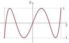
The Chebyshev polynomial T_5 = 16X5 - 20X3 + 5X on ∈tcc-11: it oscillates exactly between -1 and 1, touching the bounds at six points (marked). This equioscillation is what makes 2-4T_5 the monic quintic of smallest sup-norm on the interval ( and the weekend problem). — The Chebyshev polynomial $T_5 = 16X^5 - 20X^3 + 5X$ on $\intcc{-1}1$ : it oscillates exactly between $-1$ and $1$ , touching the bounds at six points (marked). This *equioscillation* is what makes $2^{-4}T_5$ the monic quintic of smallest sup-norm on the interval (Exercise 8.10 and the weekend problem).

Remark 8.18 (Common pitfalls with polynomials)

Polynomial versus function. Over $K = \Q, \R, \C$ the two notions match (equal functions have equal coefficients, by Corollary 8.8 and infiniteness of $K$ ), but conceptually a polynomial is its coefficient list: over the two-element field $\Z/2\Z$ of Chapter 7, $X^2 + X$ vanishes at both points, yet is not the zero polynomial.
Degrees under addition. $\deg(P + Q)$ can drop below $\max(\deg P, \deg Q)$ when leading terms cancel; writing “ $\deg(P + Q) = \max(\dots)$ ” is only safe for distinct degrees.
Roots counted correctly. “ $n$ roots” in Corollary 8.16 means with multiplicity, in $\C$ : $X^2 + 1$ has no real roots, and $(X-1)^2$ has one distinct root but two with multiplicity. Statements mixing the three counts are the commonest source of false proofs.
Irreducibility depends on the field. $X^2 - 2$ is irreducible over $\Q$ , splits over $\R$ ; $X^2 + 1$ is irreducible over $\R$ , splits over $\C$ . The bare word “irreducible” means nothing until the coefficient field is named.

8.3 Coefficients and roots

Theorem 8.19 (Vieta’s formulas)

Let $P = X^n + c_{n-1} X^{n-1} + \dots + c_0$ be monic with roots $a_1, \dots, a_n \in \C$ (with multiplicity). Then

\sum_i a_i = -c_{n-1}, \qquad \sum_{i < j} a_i a_j = c_{n-2}, \qquad \dots, \qquad a_1 a_2 \cdots a_n = (-1)^n c_0 ,

the $k$ -th symmetric function of the roots being $(-1)^k c_{n-k}$ .

Proof. By Corollary 8.16, $P = (X - a_1)\cdots(X - a_n)$ (monic, all roots listed). Expanding the product distributively produces one term per way of choosing, in each factor, either $X$ or the root term $-a_i$ : choosing the roots in the factors indexed by $i_1 < \dots < i_k$ and $X$ in the $n - k$ others contributes $(-a_{i_1})\cdots(-a_{i_k})\,X^{n-k}$ . Grouping by the power of $X$ :

P = \sum_{k=0}^{n} (-1)^k \Bigl(\sum_{i_1 < \dots < i_k} a_{i_1}\cdots a_{i_k}\Bigr) X^{n-k} ,

and identifying with $P = \sum_k c_{n-k}X^{n-k}$ (coefficients are unique, Definition 8.1) gives $c_{n-k} = (-1)^k \sigma_k$ , i.e. $\sigma_k = (-1)^kc_{n-k}$ , where $\sigma_k$ denotes the $k$ -th symmetric function displayed above. The three displayed cases are $k = 1$ , $k = 2$ and $k = n$ . ∎

Example 8.20

For the quadratic $X^2 - sX + p$ : sum of roots $s$ , product $p$ — already used repeatedly (Exercise 3.8). For a monic cubic $X^3 + aX^2 + bX + c$ with roots $\alpha, \beta, \gamma$ :

\alpha + \beta + \gamma = -a, \quad \alpha\beta + \beta\gamma + \gamma\alpha = b, \quad \alpha\beta\gamma = -c ,

which allows computing symmetric quantities like $\alpha^2 + \beta^2 + \gamma^2 = a^2 - 2b$ without solving.

Example 8.21 (Transforming the roots without finding them)

Let $\alpha, \beta$ be the roots of $X^2 - 3X + 1$ . Which monic quadratic has roots $\alpha^2, \beta^2$ ? By Vieta, $\alpha + \beta = 3$ and $\alpha\beta = 1$ , so

\alpha^2 + \beta^2 = (\alpha+\beta)^2 - 2\alpha\beta = 7, \qquad \alpha^2\beta^2 = (\alpha\beta)^2 = 1 :

the answer is $X^2 - 7X + 1$ — obtained without computing $\alpha = \frac{3 + \sqrt5}2$ . (Check: $\alpha^2 = \frac{7 + 3\sqrt5}2$ and indeed $\alpha^2 + \beta^2 = 7$ .) The same strategy handles reciprocals ( $X^2 - \frac ba X + \frac ca$ -type transformations), shifts, and any symmetric data: Vieta converts questions about unknown roots into algebra on known coefficients. It will serve constantly when the roots are eigenvalues (Chapter 22).

Example 8.22 (Palindromic equations)

Solve $X^4 + X^3 - 4X^2 + X + 1 = 0$ . The coefficients read the same in both directions, so $0$ is not a root and dividing by $X^2$ loses no solutions:

X^2 + X - 4 + \frac1X + \frac1{X^2} = 0 .

Set $y = X + \frac1X$ : then $X^2 + \frac1{X^2} = y^2 - 2$ , and the equation collapses to

y^2 + y - 6 = 0 \iff (y + 3)(y - 2) = 0 .

Unfold each value through $X^2 - yX + 1 = 0$ : for $y = 2$ , $X^2 - 2X + 1 = (X - 1)^2$ gives the double root $1$ ; for $y = -3$ , $X^2 + 3X + 1 = 0$ gives $X = \frac{-3 \pm \sqrt5}2$ . Four roots with multiplicity for a quartic, as Corollary 8.16 requires — obtained by solving two quadratics. The trick covers every palindromic polynomial: their roots come in reciprocal pairs $\{x, 1/x\}$ (replace $X$ by $1/X$ and clear denominators), and $y = X + \frac1X$ is precisely the quantity constant on such pairs, halving the degree.

Theorem 8.23 (Lagrange interpolation)

Let $x_0, \dots, x_n$ be distinct points of $K$ and $y_0, \dots, y_n \in K$ . There is exactly one $P \in K[X]$ of degree $\leq n$ with $P(x_i) = y_i$ for all $i$ , namely

P = \sum_{i=0}^{n} y_i\, L_i, \qquad L_i = \prod_{j \neq i} \frac{X - x_j}{x_i - x_j} .

Proof. Each $L_i$ has degree $n$ and satisfies $L_i(x_i) = 1$ , $L_i(x_j) = 0$ for $j \neq i$ (each factor vanishes at the corresponding $x_j$ ). So the displayed $P$ has degree $\leq n$ and interpolates. Uniqueness: two interpolating polynomials of degree $\leq n$ agree at the $n+1$ points $x_i$ , hence are equal (Corollary 8.8). ∎

Remark 8.24 (Interlude: polynomials are also vectors)

A change of viewpoint that Chapter 18 will make official: the polynomials of degree $\leq n$ form a space in which addition and scaling behave exactly like coordinates — a polynomial is its list of $n + 1$ coefficients. Three statements of this chapter are secretly linear algebra. Lagrange interpolation (Theorem 8.23) says that the evaluation data $(P(x_0), \dots, P(x_n))$ determines $P$ uniquely: evaluation at $n + 1$ points is a linear bijection, and the $L_i$ are the basis adapted to it. The expansion $R = \sum c_k(X - a)^k$ in the proof of Proposition 8.11 says that the powers of $(X - a)$ form another coordinate system, with $c_k = R^{(k)}(a)/k!$ as coordinates. And Corollary 8.8 — more roots than the degree forces the zero polynomial — is the engine of all uniqueness: it will become “a linear map injective on a space of dimension $n + 1$ ” in Chapter 19. When those chapters arrive, the space $K_n[X]$ will be their favorite example; it is worth arriving there already fluent in it.

Remark 8.25 (Where this chapter is used)

Factorization over $\R$ and $\C$ (Corollary 8.16) is the engine of partial fractions in Chapter 9, hence of a large class of integrals in Chapter 15. The expansion of a polynomial in powers of $(X - a)$ , met in the proof of Proposition 8.11, is the algebraic shadow of the Taylor formulas of Chapter 16. Characteristic polynomials already appeared for differential equations (Chapter 5) and return for matrices in Chapter 22; Lagrange interpolation is the first existence-and-uniqueness theorem of numerical analysis, and the Chebyshev polynomials of Exercise 8.10 — whose optimality the weekend problem below establishes — tell that discipline where to interpolate. Finally the whole arithmetic of $K[X]$ , copied from Chapter 6, feeds the study of $K[X]$ -ideals and quotient rings in the Year 2 volume.

8.4 Exercises

Exercise 8.1 ★

Carry out the Euclidean divisions: $X^5 - 1$ by $X^2 + X + 1$ ; then $2X^4 + X^3 - X + 3$ by $X^2 - 2$ .

Solution

Solution of Exercise 8.1.

$X^5 - 1 = (X^2 + X + 1)(X^3 - X^2 + 1) + (-X - 2)$ . Steps: subtract $X^3 B$ , then $-X^2 B$ , then $B$ ; the remainder $-X - 2$ has degree $1 < 2$ . Check at $X = 1$ : $\;0 = 3 \times 1 + (-3)$ .

$2X^4 + X^3 - X + 3 = (X^2 - 2)(2X^2 + X + 4) + (X + 11)$ . Check at $X = 0$ : $\;3 = (-2)(4) + 11$ .

Exercise 8.2 ★

For which $n \in \N$ does $X^2 + X + 1$ divide $X^{2n} + X^n + 1$ ? Hint: the roots of $X^2 + X + 1$ are $j$ and $j^2$ with $j = \eu^{2\iu\pi/3}$ ; discuss $n$ mod $3$ .

Solution

Solution of Exercise 8.2.

$X^2 + X + 1 = (X - j)(X - j^2)$ with $j = \eu^{2\iu\pi/3}$ , $j^3 = 1$ . It divides $Q_n = X^{2n} + X^n + 1$ iff $j$ and $j^2$ are roots of $Q_n$ ; since $Q_n$ has real coefficients, $Q_n(j^2) = \conj{Q_n(j)}$ , so the condition is just $Q_n(j) = 0$ . Now $Q_n(j) = j^{2n} + j^n + 1$ depends on $n$ mod $3$ :

$n \equiv 0$ : $Q_n(j) = 1 + 1 + 1 = 3 \neq 0$ ;
$n \equiv 1$ : $Q_n(j) = j^2 + j + 1 = 0$ ;
$n \equiv 2$ : $Q_n(j) = j^4 + j^2 + 1 = j + j^2 + 1 = 0$ .

So $X^2 + X + 1 \mid X^{2n} + X^n + 1$ exactly when $3 \nmid n$ .

Exercise 8.3 ★

Determine the real $a, b$ so that $(X-1)^2$ divides $P = X^4 + aX^3 + bX^2 + 1$ , then factor $P$ over $\R$ for these values.

Solution

Solution of Exercise 8.3.

By Proposition 8.11, $(X-1)^2 \mid P$ iff $P(1) = P'(1) = 0$ :

P(1) = 2 + a + b = 0, \qquad P'(1) = 4 + 3a + 2b = 0 .

Solving: $b = -a - 2$ and $4 + 3a - 2a - 4 = a = 0$ , so $a = 0$ , $b = -2$ : $P = X^4 - 2X^2 + 1 = (X^2 - 1)^2 = (X-1)^2 (X+1)^2$ , which is the real factorization.

Exercise 8.4 ★

Factor over $\C$ and over $\R$ : $X^3 - 1$ ; $\;X^4 + X^2 + 1$ ; $\;X^6 - 1$ .

Solution

Solution of Exercise 8.4.

$X^3 - 1 = (X - 1)(X - j)(X - j^2)$ over $\C$ ( $j = \eu^{2\iu\pi/3}$ ), and $(X - 1)(X^2 + X + 1)$ over $\R$ .

$X^4 + X^2 + 1 = (X^2 + X + 1)(X^2 - X + 1)$ over $\R$ (multiply out, or note $X^4 + X^2 + 1 = (X^2+1)^2 - X^2$ ); over $\C$ , each quadratic splits: roots $j, j^2$ and $-j, -j^2$ , i.e. $\eu^{\pm 2\iu\pi/3}, \eu^{\pm\iu\pi/3}$ .

$X^6 - 1 = \prod_{k=0}^{5} (X - \eu^{\iu k\pi/3})$ over $\C$ , and over $\R$ :

X^6 - 1 = (X-1)(X+1)(X^2 + X + 1)(X^2 - X + 1),

grouping the conjugate pairs $\eu^{\pm 2\iu\pi/3}$ and $\eu^{\pm \iu\pi/3}$ .

Exercise 8.5 ★★

Let $P = X^3 - 6X^2 + 11X - 6$ .

Find the rational roots (a rational root $p/q$ in lowest terms of a monic integer polynomial is an integer dividing the constant term — prove it), and factor $P$ .
Without solving, compute the sum of the squares and the sum of the inverses of the roots via Vieta, and check on the factorization.

Solution

Solution of Exercise 8.5.

Let $p/q$ (lowest terms) be a root of the monic integer polynomial $X^3 + \dots + c_0$ : clearing denominators in $P(p/q) = 0$ gives $p^3 = -q\,(\text{integer})$ , so $q \mid p^3$ ; coprimality forces $q = \pm 1$ : the root is an integer $p$ , and $p \mid c_0$ (isolate $c_0$ ). Here the candidates divide $6$ : testing, $P(1) = 0$ , $P(2) = 0$ , $P(3) = 0$ . So $P = (X-1)(X-2)(X-3)$ .
Vieta: $s_1 = 6$ , $s_2 = 11$ , $s_3 = 6$ . Sum of squares: $s_1^2 - 2s_2 = 36 - 22 = 14 = 1 + 4 + 9$ , as expected. Sum of inverses: $\frac{s_2}{s_3} = \frac{11}{6} = 1 + \frac12 + \frac13$ , as expected.

Exercise 8.6 ★★

Compute $\gcd(X^4 - 1,\; X^3 - X^2 + X - 1)$ by the Euclidean algorithm, and write it as a combination $AU + BV$ of the two polynomials.

Solution

Solution of Exercise 8.6.

First division step of the Euclidean algorithm:

(X + 1)(X^3 - X^2 + X - 1) = X^4 - X^3 + X^2 - X + X^3 - X^2 + X - 1 = X^4 - 1 ,

so the division of $X^4 - 1$ by $X^3 - X^2 + X - 1$ is exact (quotient $X + 1$ , remainder $0$ ), and the algorithm stops at once:

\gcd(X^4 - 1,\; X^3 - X^2 + X - 1) = X^3 - X^2 + X - 1

(already monic). The Bézout relation is the trivial one: $\gcd = 0 \cdot (X^4 - 1) + 1 \cdot (X^3 - X^2 + X - 1)$ . Consistency check by factoring: $X^3 - X^2 + X - 1 = (X - 1)(X^2 + 1)$ , which is indeed the product of the common irreducible factors of $X^4 - 1 = (X-1)(X+1)(X^2+1)$ .

Exercise 8.7 ★★

Let $P \in \R[X]$ with $P(x) \geq 0$ for all $x \in \R$ . Prove that $P$ is a sum of two squares of real polynomials: $P = A^2 + B^2$ . Hint: in the real factorization, real roots have even multiplicity; write the quadratic factors as $(X - z)(X - \conj z)$ and use $\abs{\,\cdot\,}^2 = (\Re)^2 + (\Im)^2$ on the product of the $(X - z)$ ’s.

Solution

Solution of Exercise 8.7.

Since $P \geq 0$ on $\R$ , its real roots have even multiplicity (at a root of odd multiplicity, $P$ changes sign). Using Corollary 8.16 and pairing, write

P = c \prod_i (X - a_i)^{2k_i} \prod_j \bigl((X - z_j)(X - \conj z_j)\bigr)^{n_j},

with $c > 0$ (behavior at $+\infty$ ). Let

S = \sqrt c\, \prod_i (X - a_i)^{k_i} \prod_j (X - z_j)^{n_j} \in \C[X],

so that $P = S\,\conj S$ where $\conj S$ has the conjugated coefficients. Split $S = A + \iu B$ with $A, B \in \R[X]$ : then

P = (A + \iu B)(A - \iu B) = A^2 + B^2 .

Exercise 8.8 ★★

Find the polynomial $P$ of degree $\leq 2$ with $P(0) = 1$ , $P(1) = 3$ , $P(2) = 2$ , first by Lagrange’s formula, then by solving the linear system on the coefficients. Verify both answers agree.

Solution

Solution of Exercise 8.8.

Lagrange (Theorem 8.23) with nodes $0, 1, 2$ :

P = 1\cdot\frac{(X-1)(X-2)}{(0-1)(0-2)} + 3\cdot\frac{X(X-2)}{1\cdot(1-2)} + 2\cdot\frac{X(X-1)}{2\cdot 1} = \frac{(X-1)(X-2)}{2} - 3X(X-2) + X(X-1).

Expanding: $\frac{X^2 - 3X + 2}{2} - 3X^2 + 6X + X^2 - X = -\frac{3}{2}X^2 + \frac{7}{2}X + 1$ .

System: $P = aX^2 + bX + c$ with $c = 1$ ; $a + b + 1 = 3$ ; $4a + 2b + 1 = 2$ . Subtracting twice the second from the third: $2a - 1 = -4$ , so $a = -\frac32$ , $b = \frac72$ . Same polynomial: $P = -\frac32 X^2 + \frac72 X + 1$ . (Check $P(2) = -6 + 7 + 1 = 2$ .)

Exercise 8.9 ★★

Prove that $P = X^{2n+1} - 1$ has exactly one real root, and that for every $n \geq 1$ the polynomial $1 + X + \frac{X^2}{2!} + \dots + \frac{X^n}{n!}$ has no multiple root (compare $P$ and $P'$ ).

Solution

Solution of Exercise 8.9.

$P = X^{2n+1} - 1$ : $P' = (2n+1)X^{2n} \geq 0$ , so the polynomial function is increasing (strictly except at $0$ ), with limits $\mp\infty$ : it vanishes exactly once on $\R$ (at $x = 1$ ).

Let $E_n = \sum_{k=0}^{n} \frac{X^k}{k!}$ . Then $E_n' = E_{n-1} = E_n - \frac{X^n}{n!}$ . A multiple root $a$ would satisfy $E_n(a) = E_n'(a) = 0$ (Proposition 8.11), hence $\frac{a^n}{n!} = E_n(a) - E_n'(a) = 0$ , so $a = 0$ ; but $E_n(0) = 1 \neq 0$ . No multiple root.

Exercise 8.10 ★★★

(Chebyshev polynomials) Define $T_0 = 1$ , $T_1 = X$ and $T_{n+1} = 2X\,T_n - T_{n-1}$ .

Prove by induction that $T_n(\cos\theta) = \cos n\theta$ for all $\theta$ .
Deduce the $n$ roots of $T_n$ and its leading coefficient.
Prove that $\sup_{x \in \intcc{-1}{1}} \abs{T_n(x)} = 1$ , attained at $n + 1$ points of $\intcc{-1}{1}$ .

Solution

Solution of Exercise 8.10.

Induction (two base cases hold). Using $\cos(n+1)\theta + \cos(n-1)\theta = 2\cos\theta\cos n\theta$ :

$T_{n+1}(\cos\theta) = 2\cos\theta \cos n\theta - \cos(n-1)\theta = \cos(n+1)\theta .$
$T_n(\cos\theta) = 0$ iff $n\theta \equiv \frac\pi2 \pmod \pi$ : the numbers

$x_k = \cos\Bigl(\frac{(2k+1)\pi}{2n}\Bigr), \qquad k = 0, 1, \dots, n-1,$

are $n$ distinct points of $\intoo{-1}{1}$ (the angles lie in $\intoo{0}{\pi}$ where $\cos$ is injective), all roots of $T_n$ ; since $\deg T_n = n$ (from the recurrence, with leading coefficient $2^{n-1}$ for $n \geq 1$ , by induction), these are all the roots, each simple.
For $x = \cos\theta \in \intcc{-1}{1}$ : $\abs{T_n(x)} = \abs{\cos n\theta} \leq 1$ , with equality iff $n\theta \equiv 0 \pmod\pi$ , i.e. at the $n+1$ points $y_k = \cos\frac{k\pi}{n}$ , $k = 0, \dots, n$ , where $T_n(y_k) = (-1)^k$ . (This equioscillation makes $2^{1-n}T_n$ the monic degree- $n$ polynomial of smallest sup-norm on $\intcc{-1}{1}$ — proved in this chapter’s weekend problem.)

Exercise 8.11 ★★★

Let $P \in \C[X]$ be nonconstant with distinct roots $a_1, \dots, a_r$ (multiplicities $m_1, \dots, m_r$ ). Prove the identity of rational functions

\frac{P'(X)}{P(X)} = \sum_{i=1}^{r} \frac{m_i}{X - a_i},

and deduce the Gauss–Lucas theorem: every root of $P'$ lies in the convex hull of the roots of $P$ (evaluate the identity at a root $w$ of $P'$ which is not a root of $P$ , take conjugates, and read the result as $w$ being a weighted average of the $a_i$ ).

Solution

Solution of Exercise 8.11.

Write $P = c\prod_i (X - a_i)^{m_i}$ . The product rule (extended to several factors) gives

P' = c\sum_{i} m_i (X - a_i)^{m_i - 1} \prod_{k \neq i} (X - a_k)^{m_k},

and dividing by $P$ : $\frac{P'}{P} = \sum_i \frac{m_i}{X - a_i}$ (as rational functions, i.e. away from the roots).

Let $w$ be a root of $P'$ . If $w$ is one of the $a_i$ , it lies in the convex hull trivially. Otherwise, evaluating at $w$ :

0 = \sum_i \frac{m_i}{w - a_i} = \sum_i m_i\, \frac{\conj w - \conj a_i}{\abs{w - a_i}^2} .

Conjugating: $\sum_i \lambda_i (w - a_i) = 0$ where $\lambda_i = \frac{m_i}{\abs{w - a_i}^2} > 0$ . Hence

w = \frac{\sum_i \lambda_i a_i}{\sum_i \lambda_i} :

a convex combination (positive weights summing to $1$ after normalization) of the roots $a_i$ . So every root of $P'$ lies in the convex hull of the roots of $P$ .

Exercise 8.12 ★★

(Roots-of-unity filter) Let $n \in \N^*$ and $j = \eu^{2\iu\pi/3}$ . Evaluating $(1 + X)^n$ at $1$ , $j$ and $j^2$ , prove that

\sum_{k \geq 0} \binom{n}{3k} = \frac{2^n + 2\cos\frac{n\pi}{3}}{3} ,

and check the formula for $n = 3$ and $n = 6$ . Hint: $1 + j^m + j^{2m}$ equals $3$ if $3 \mid m$ and $0$ otherwise; and $1 + j = \eu^{\iu\pi/3}$ .

Solution

Solution of Exercise 8.12.

Sum the evaluations of $(1 + X)^n$ at the three cube roots of unity:

2^n + (1 + j)^n + (1 + j^2)^n = \sum_{k=0}^n \binom nk\,\bigl(1 + j^k + j^{2k}\bigr) = 3\sum_{k\,:\,3\mid k}\binom nk ,

since $1 + j^k + j^{2k}$ is a geometric sum equal to $3$ when $3 \mid k$ and to $\frac{j^{3k} - 1}{j^k - 1} = 0$ otherwise. Now $1 + j = \frac12 + \iu\frac{\sqrt3}2 = \eu^{\iu\pi/3}$ and $1 + j^2 = \conj{1 + j} = \eu^{-\iu\pi/3}$ , so $(1+j)^n + (1+j^2)^n = 2\cos\frac{n\pi}3$ and

\sum_{k\geq0}\binom n{3k} = \frac{2^n + 2\cos\frac{n\pi}3}{3} .

Checks: $n = 3$ : $\frac{8 + 2\cos\pi}3 = 2 = \binom30 + \binom33$ ; $n = 6$ : $\frac{64 + 2}3 = 22 = 1 + 20 + 1$ .

8.5 Problem: Chebyshev polynomials and the flattest polynomial

Problem 8.1

Among all monic polynomials of degree $n$ , which one stays closest to zero on $\intcc{-1}1$ ? The answer — Chebyshev’s theorem, the birth certificate of approximation theory — is $2^{1-n}T_n$ , where $T_n$ is the Chebyshev polynomial of Exercise 8.10, and no monic competitor can beat its deviation $2^{1-n}$ . This problem develops the algebra of the family $(T_n)$ (composition law, explicit coefficients, the second-kind family $U_n$ , a differential equation), proves the extremality theorem with its equality case, and collects applications: optimal interpolation nodes, the exact value of $\cos 36^\circ$ , and a congruence $T_p \equiv X^p \pmod p$ . Throughout, $T_0 = 1$ , $T_1 = X$ , $T_{n+1} = 2X\,T_n - T_{n-1}$ , and we freely use $T_n(\cos\theta) = \cos n\theta$ from Exercise 8.10.

Part I — The family $(T_n)$ .

Compute $T_2, T_3, T_4, T_5$ from the recurrence. (Compare $T_3$ with the identity $\cos3\theta = 4\cos^3\theta - 3\cos\theta$ of Example 3.9.)
Prove by induction: $\deg T_n = n$ with leading coefficient $2^{n-1}$ for $n \geq 1$ , and $T_n$ has the parity of $n$ (only even or only odd powers appear).
Prove the uniqueness principle: $T_n$ is the only polynomial satisfying $P(\cos\theta) = \cos n\theta$ for all $\theta$ . (Two polynomials agreeing on $\intcc{-1}1$ agree everywhere: Corollary 8.8.)
Deduce the composition and product laws:

$T_m \circ T_n = T_{mn}, \qquad 2\,T_m T_n = T_{m+n} + T_{\abs{m-n}} .$
Recall from Exercise 8.10 the roots $x_k = \cos\frac{(2k+1)\pi}{2n}$ and the equioscillation points $y_k = \cos\frac{k\pi}n$ with $T_n(y_k) = (-1)^k$ . Write down the complete factorization of $T_n$ over $\R$ , and justify that the $y_k$ interlace: $y_n < x_{n-1} < y_{n-1} < \dots < x_0 < y_0$ .
Prove that $T_n(\cosh t) = \cosh(nt)$ for all $t \in \R$ (same induction, using Proposition 4.18), and deduce for $x \geq 1$ the closed form

$T_n(x) = \frac{\bigl(x + \sqrt{x^2 - 1}\bigr)^n + \bigl(x - \sqrt{x^2 - 1}\bigr)^n}{2} ,$

so $T_n(x) > 1$ for $x > 1$ : outside $\intcc{-1}1$ the polynomial escapes at once.

Part II — Coefficients, the family $U_n$ , a differential equation.

From de Moivre’s formula (Corollary 3.8), prove the explicit expression

$T_n(x) = \sum_{0 \leq 2j \leq n} \binom{n}{2j}\, x^{\,n-2j}\,(x^2 - 1)^j ,$

and verify it for $n = 3$ .
Compute $T_n(1)$ , $T_n(-1)$ and $T_n(0)$ for all $n$ .
Define $U_n$ (second kind) by $U_0 = 1$ , $U_1 = 2X$ , $U_{n+1} = 2X\,U_n - U_{n-1}$ . Prove that $U_n(\cos\theta) = \frac{\sin(n+1)\theta}{\sin\theta}$ for $\theta \notin \pi\Z$ , and that $T_n' = n\,U_{n-1}$ for $n \geq 1$ .
Prove that $\abs{\sin n\theta} \leq n\,\abs{\sin\theta}$ for all $\theta$ (induction), and deduce the Markov-type bound

$\abs{T_n'(x)} \leq n^2 \quad\text{on } \intcc{-1}1, \qquad\text{with } T_n'(\pm1) = (\pm1)^{n-1}\,n^2 .$
Show that $y = T_n$ satisfies the differential equation

$(1 - x^2)\,y'' - x\,y' + n^2\,y = 0 ,$

by differentiating the identity $\sin\theta\, T_n'(\cos\theta) = n\sin n\theta$ with respect to $\theta$ ; verify directly for $T_2$ .

Part III — Chebyshev’s extremality theorem. Let $\widetilde T_n = 2^{1-n}\,T_n$ (monic by question 2) and write $\norm{P}_\infty = \sup_{x \in \intcc{-1}1}\abs{P(x)}$ .

Justify $\norm{\widetilde T_n}_\infty = 2^{1-n}$ , attained with alternating signs at the $n + 1$ points $y_n < \dots < y_0$ .
Suppose some monic $P$ of degree $n$ had $\norm P_\infty < 2^{1-n}$ , and set $D = \widetilde T_n - P$ . Show $\deg D \leq n - 1$ , and that $D(y_k)$ has the strict sign of $(-1)^k$ for each $k = 0, \dots, n$ .
Deduce that $D$ has at least $n$ distinct real roots (one in each gap, by the intermediate value property, used here at High School level and proved in Chapter 13), and conclude Chebyshev’s theorem: every monic $P$ of degree $n$ satisfies

$\norm{P}_\infty \geq 2^{1-n} .$
(Equality case, first step) Suppose now $\norm P_\infty = 2^{1-n}$ exactly, $P$ monic of degree $n$ , and let $D = \widetilde T_n - P$ . Show that $(-1)^kD(y_k) \geq 0$ for all $k$ , and that if $D(y_k) = 0$ for an interior point $y_k$ ( $0 < k < n$ ), then $D'(y_k) = 0$ as well. (At an interior $y_k$ , both $\widetilde T_n$ and $P$ attain an extremum of absolute value $\norm{\cdot} _\infty$ ; a differentiable function has zero derivative at an interior extremum — used at High School level, proved in Chapter 14.)
(Equality case, conclusion) Count roots of $D$ with multiplicity to show $D = 0$ : the minimizer is unique, $P = \widetilde T_n$ .
Transport to an arbitrary segment $\intcc ab$ : show that the minimal sup-norm of a monic degree- $n$ polynomial on $\intcc ab$ is $2\bigl(\frac{b-a}4\bigr)^n$ , attained by a rescaled Chebyshev polynomial. (Substitute $x = \frac{a+b}2 + \frac{b-a}2\,t$ and track the leading coefficient.)

Part IV — Applications.

Work out the case $n = 3$ by hand: locate the extrema of $\widetilde T_3 = X^3 - \frac34X$ on $\intcc{-1}1$ , verify the four-fold equioscillation with value $\frac14$ , and conclude that no monic cubic does better.
(Optimal interpolation nodes) For $n + 1$ nodes $x_0, \dots, x_n \in \intcc{-1}1$ , the interpolation error is governed by $\omega(X) = \prod_i (X - x_i)$ (as Chapter 16 will quantify). Prove that the choice minimizing $\norm\omega_\infty$ is the set of $n + 1$ roots of $T_{n+1}$ , with $\norm\omega_\infty = 2^{-n}$ : Chebyshev nodes are the right places to interpolate.
Using $T_5$ , prove that $c = \cos 36^\circ$ satisfies $16c^5 - 20c^3 + 5c + 1 = 0$ , factor this polynomial as $(x + 1)(4x^2 - 2x - 1)^2$ , and conclude

$\cos 36^\circ = \frac{1 + \sqrt5}4 .$

Check the consistency with $\cos 72^\circ = \frac{\sqrt5 - 1}4$ from Exercise 3.8.
Estimate $T_{10}(1.1)$ with the closed form of question 6 (two significant digits suffice), and interpret: a polynomial bounded by $1$ on $\intcc{-1}1$ can already exceed $40$ at $x = 1.1$ . (That $T_n$ grows fastest among such polynomials is another extremal property of the family, beyond this problem.)
Prove the congruence: for every odd prime $p$ , all coefficients of $T_p - X^p$ are divisible by $p$ . (Use question 7 and $p \mid \binom p{2j}$ for $0 < 2j < p$ , from the proof of Theorem 6.23.) Verify on $T_3$ and $T_5$ .

Part V — Synthesis.

Compute explicitly the monic quadratic of minimal sup-norm on $\intcc01$ and its deviation. (Question 17 with $n = 2$ .)
Where exactly did the problem use: (i) the rigidity of polynomials (Corollary 8.8); (ii) the trigonometry of Chapter 3 and Chapter 4; (iii) the arithmetic of binomial coefficients from Chapter 6? One sentence each.
Synthesis, in a short paragraph: the theorem says that the flattest monic polynomial is the one that equioscillates, and the proof converts optimality into root-counting. Comment on this mechanism, on the role of the substitution $x = \cos\theta$ as a bridge between algebra and trigonometry, and name the two places where the problem needed analysis facts (IVT, interior extremum) that later chapters prove.

Solution

Solution of Problem 8.1.

1. $T_2 = 2X^2 - 1$ ; $T_3 = 2X(2X^2 - 1) - X = 4X^3 - 3X$ ; $T_4 = 2X\,T_3 - T_2 = 8X^4 - 8X^2 + 1$ ; $T_5 = 2X\,T_4 - T_3 = 16X^5 - 20X^3 + 5X$ . The identity $T_3(\cos\theta) = \cos3\theta$ is exactly $\cos3\theta = 4\cos^3\theta - 3\cos\theta$ from Example 3.9.

2. True for $n = 1, 2$ . If $T_{n-1}$ , $T_n$ have degrees $n-1$ , $n$ and leading coefficients $2^{n-2}$ , $2^{n-1}$ , then $2X\,T_n$ has degree $n+1$ and leading coefficient $2^n$ , while $T_{n-1}$ has lower degree: $T_{n+1}$ has degree $n + 1$ , leading coefficient $2^n$ . Parity: if $T_{n-1}$ has the parity of $n - 1$ and $T_n$ that of $n$ , then $2X\,T_n$ and $T_{n-1}$ both have the parity of $n + 1$ , hence so does $T_{n+1}$ .

3. If $P(\cos\theta) = \cos n\theta$ for all $\theta$ , then $P$ and $T_n$ agree at every point of $\intcc{-1}1$ — an infinite set — so $P - T_n$ has infinitely many roots and is the zero polynomial (Corollary 8.8).

4. For $x = \cos\theta$ : $T_m(T_n(\cos\theta)) = T_m(\cos n\theta) = \cos(mn\theta) = T_{mn}(\cos\theta)$ , and $2T_mT_n(\cos\theta) = 2\cos m\theta\cos n\theta = \cos(m+n)\theta + \cos\abs{m - n}\theta$ . Both identities hold on $\intcc{-1}1$ , hence as polynomial identities by question 3’s argument.

5. The $x_k$ are $n$ distinct simple roots and the leading coefficient is $2^{n-1}$ :

T_n = 2^{n-1}\prod_{k=0}^{n-1} \Bigl(X - \cos\frac{(2k+1)\pi}{2n}\Bigr) .

Interlacing: the angles $0 < \frac{\pi}{2n} < \frac\pi n < \frac{3\pi}{2n} < \frac{2\pi}n < \dots < \pi$ alternate between the $y$ -angles $\frac{k\pi}n$ and the $x$ -angles $\frac{(2k+1)\pi}{2n}$ ; since $\cos$ is strictly decreasing on $\intcc0\pi$ , the values interlace in the reverse order: $y_n < x_{n-1} < y_{n-1} < \dots < x_0 < y_0$ . Between two consecutive extrema sits exactly one root, as a picture of $\cos n\theta$ suggests.

6. Induction with $2\cosh a\cosh b = \cosh(a + b) + \cosh(a - b)$ (Proposition 4.18): $T_{n+1}(\cosh t) = 2\cosh t\cosh nt - \cosh(n-1)t = \cosh(n+1)t$ . For $x \geq 1$ , write $x = \cosh t$ with $t \geq 0$ ; then $\eu^t = x + \sqrt{x^2 - 1}$ and $\eu^{-t} = x - \sqrt{x^2 - 1}$ , so

T_n(x) = \cosh(nt) = \frac{(x + \sqrt{x^2-1})^n + (x - \sqrt{x^2-1})^n}2 .

For $x > 1$ the first term exceeds $\frac12(1)^n$ strictly and grows geometrically: $T_n(x) > 1$ .

7. De Moivre: $\cos n\theta = \Re\bigl((\cos\theta + \iu\sin\theta)^n\bigr) = \sum_{2j \leq n}\binom n{2j} \cos^{n-2j}\theta\,(\iu\sin\theta)^{2j}$ , and $(\iu\sin\theta)^{2j} = (-\sin^2\theta)^j = (\cos^2\theta - 1)^j$ . Substituting $x = \cos\theta$ and invoking question 3:

T_n(x) = \sum_{0\leq 2j\leq n}\binom n{2j}x^{n-2j}(x^2 - 1)^j .

For $n = 3$ : $\binom30 x^3 + \binom32 x(x^2 - 1) = x^3 + 3x^3 - 3x = 4x^3 - 3x$ , as in question 1.

8. $T_n(1) = \cos(n\cdot0) = 1$ ; $T_n(-1) = \cos(n\pi) = (-1)^n$ ; $T_n(0) = \cos\frac{n\pi}2$ , which is $0$ for odd $n$ and $(-1)^{n/2}$ for even $n$ .

9. Induction for $U_n(\cos\theta) = \frac{\sin(n+1)\theta}{\sin\theta}$ : true for $U_0 = 1$ and $U_1 = 2X$ ( $\sin2\theta = 2\sin\theta\cos\theta$ ); the step is the sum-to-product identity $\sin(n+2)\theta = 2\cos\theta\, \sin(n+1)\theta - \sin n\theta$ . Now differentiate $T_n(\cos\theta) = \cos n\theta$ in $\theta$ : $-\sin\theta\,T_n'(\cos\theta) = -n\sin n\theta$ , so for $\theta \notin \pi\Z$ :

T_n'(\cos\theta) = n\,\frac{\sin n\theta}{\sin\theta} = n\,U_{n-1}(\cos\theta) ,

and the polynomials $T_n'$ and $nU_{n-1}$ , agreeing on $\intoo{-1}1$ , are equal.

10. $\abs{\sin(n+1)\theta} = \abs{\sin n\theta\cos\theta + \cos n\theta\sin\theta} \leq \abs{\sin n\theta} + \abs{\sin\theta}$ , and induction gives $\abs{\sin n\theta} \leq n\abs{\sin\theta}$ . Hence $\abs{U_{n-1}} \leq n$ on $\intoo{-1}1$ and $\abs{T_n'} = n\abs{U_{n-1}} \leq n^2$ there; at $\pm1$ the bound extends by taking limits (or directly: $U_{n-1}(1) = n$ from the recurrence, $U_n(1) = n + 1$ by induction, and parity gives $U_{n-1}(-1) = (-1)^{n-1}n$ ). Thus $T_n'(1) = n^2$ and $T_n'(-1) = (-1)^{n-1}n^2$ : the bound $n^2$ is attained at the endpoints.

11. Differentiate $\sin\theta\,T_n'(\cos\theta) = n\sin n\theta$ (question 9) with respect to $\theta$ :

\cos\theta\,T_n'(\cos\theta) - \sin^2\theta\,T_n''(\cos\theta) = n^2\cos n\theta = n^2\,T_n(\cos\theta) .

With $x = \cos\theta$ and $\sin^2\theta = 1 - x^2$ : $x\,T_n' - (1 - x^2)T_n'' = n^2T_n$ on $\intcc{-1}1$ , hence everywhere: $(1 - x^2)y'' - xy' + n^2y = 0$ for $y = T_n$ . Check for $T_2 = 2x^2 - 1$ : $(1 - x^2)(4) - x(4x) + 4(2x^2 - 1) = 4 - 4x^2 - 4x^2 + 8x^2 - 4 = 0$ .

12. $\widetilde T_n$ is monic (question 2) and $\abs{\widetilde T_n} = 2^{1-n}\abs{T_n} \leq 2^{1-n}$ on $\intcc{-1}1$ , with $\widetilde T_n(y_k) = (-1)^k2^{1-n}$ at the $n + 1$ points $y_k$ (Exercise 8.10): the norm is exactly $2^{1-n}$ , attained with alternating signs.

13. $\widetilde T_n$ and $P$ are both monic of degree $n$ , so the leading terms cancel: $\deg D \leq n - 1$ . At $y_k$ : $D(y_k) = (-1)^k2^{1-n} - P(y_k)$ , and $\abs{P(y_k)} \leq \norm P_\infty < 2^{1-n}$ forces the sign of $D(y_k)$ to be that of $(-1)^k2^{1-n}$ , strictly.

14. $D$ changes sign between $y_{k+1}$ and $y_k$ for each $k = 0, \dots, n-1$ : by the intermediate value property, $D$ has a root in each of these $n$ pairwise disjoint open intervals — $n$ distinct roots for a nonzero polynomial of degree $\leq n - 1$ , impossible. And $D = 0$ is impossible too (the norms differ). Contradiction: no monic $P$ of degree $n$ has $\norm P_\infty < 2^{1-n}$ , which is Chebyshev’s theorem.

15. Now $\abs{P(y_k)} \leq 2^{1-n}$ only, so $(-1)^k D(y_k) = 2^{1-n} - (-1)^kP(y_k) \geq 2^{1-n} - \abs{P(y_k)} \geq 0$ . Suppose $D(y_k) = 0$ at an interior $y_k$ ( $0 < k < n$ ): then $P(y_k) = (-1)^k2^{1-n}$ , so $\abs P$ attains its supremum $2^{1-n}$ at the interior point $y_k$ , whence $P'(y_k) = 0$ (interior extremum); and $T_n'(y_k) = nU_{n-1}(y_k) = 0$ since $\sin(n\cdot\frac{k\pi}n) = 0$ — so $\widetilde T_n'(y_k) = 0$ too, and $D'(y_k) = 0$ : $y_k$ is a root of $D$ of multiplicity at least $2$ .

16. Count roots of $D$ with multiplicity. Let $z$ be the number of interior points $y_k$ with $D(y_k) = 0$ (each a double root, by question 15) and $e \in \{0, 1, 2\}$ the number of endpoints ( $y_0$ or $y_n$ ) with $D = 0$ (each a simple root at least). A gap $(y_{k+1}, y_k)$ whose two endpoints both have $D \neq 0$ carries strictly alternating signs, hence an interior root. Each vanishing interior point spoils at most its two adjacent gaps, each vanishing endpoint at most one gap: at least $n - 2z - e$ gaps still contribute one root each, all distinct from the $y$ -roots. Total: at least $(n - 2z - e) + 2z + e = n$ roots with multiplicity, for a polynomial of degree $\leq n - 1$ : so $D = 0$ and $P = \widetilde T_n$ . The minimizer is unique.

17. The affine map $t \mapsto x = \frac{a+b}2 + \frac{b-a}2\,t$ is a bijection $\intcc{-1}1 \to \intcc ab$ . If $P$ is monic of degree $n$ , then $Q(t) = P(x(t))$ is a polynomial in $t$ with leading coefficient $\bigl(\frac{b-a}2\bigr)^n$ , and $\sup_{\intcc ab}\abs P = \sup_{\intcc{-1}1}\abs Q$ . The monic polynomial $Q/\bigl(\frac{b-a}2\bigr)^n$ has sup-norm $\geq 2^{1-n}$ (questions 13–14), so

\sup_{\intcc ab}\abs P \geq \Bigl(\frac{b-a}2\Bigr)^n 2^{1-n} = 2\Bigl(\frac{b-a}4\Bigr)^n ,

with equality exactly for $P(x) = \bigl(\frac{b-a}2\bigr)^n \widetilde T_n\bigl(t(x)\bigr)$ (question 16).

18. $\widetilde T_3 = \frac{T_3}4 = X^3 - \frac34X$ ; $\widetilde T_3{}' = 3X^2 - \frac34$ vanishes at $\pm\frac12$ . Values: $\widetilde T_3(-1) = -\frac14$ , $\widetilde T_3(-\tfrac12) = \frac14$ , $\widetilde T_3(\tfrac12) = -\frac14$ , $\widetilde T_3(1) = \frac14$ : four alternating extrema of absolute value $\frac14$ — so $\norm{\widetilde T_3}_\infty = \frac14$ , and by Chebyshev’s theorem no monic cubic has smaller sup-norm on $\intcc{-1}1$ .

19. $\omega$ is monic of degree $n + 1$ , so $\norm\omega_\infty \geq 2^{-n}$ by Chebyshev’s theorem (degree $n+1$ ), with equality if and only if $\omega = \widetilde T_{n+1} = 2^{-n}T_{n+1}$ (question 16), i.e. if and only if the nodes are the $n + 1$ roots of $T_{n+1}$ . With Chebyshev nodes the error factor $\norm\omega_\infty$ is $2^{-n}$ — the least possible.

20. $5 \times 36^\circ = 180^\circ$ , so $T_5(c) = \cos180^\circ = -1$ : $16c^5 - 20c^3 + 5c + 1 = 0$ . Testing $x = -1$ : $-16 + 20 - 5 + 1 = 0$ , and expanding confirms

16x^5 - 20x^3 + 5x + 1 = (x + 1)\bigl(4x^2 - 2x - 1\bigr)^2 .

Since $c = \cos36^\circ \neq -1$ , $c$ is a root of $4x^2 - 2x - 1$ , whose roots are $\frac{1 \pm \sqrt5}4$ ; as $c > 0$ ,

\cos36^\circ = \frac{1 + \sqrt5}4 .

Consistency: $\cos72^\circ = T_2(c) = 2c^2 - 1 = 2\cdot\frac{3 + \sqrt5}8 - 1 = \frac{\sqrt5 - 1}4$ , the value found in Exercise 3.8.

21. $\sqrt{1.1^2 - 1} = \sqrt{0.21} \approx 0.458$ , so $x + \sqrt{x^2-1} \approx 1.558$ and $(1.558)^{10} \approx 84.5$ , while $(1.1 - 0.458)^{10} \approx 0.01$ : $T_{10}(1.1) \approx \frac{84.5 + 0.01}2 \approx 42$ . A polynomial trapped in $\intcc{-1}1$ on the interval has already grown past $40$ one tenth beyond its edge: boundedness on a segment says nothing an inch outside it.

22. In question 7’s formula for $T_p$ , the term $j = 0$ is $X^p$ ; every other term carries $\binom p{2j}$ with $0 < 2j < p$ (note $2j \neq p$ since $p$ is odd), which is divisible by $p$ by the first step of the proof of Theorem 6.23. Hence every coefficient of $T_p - X^p$ is a multiple of $p$ . Checks: $T_3 - X^3 = 3X^3 - 3X = 3(X^3 - X)$ ; $T_5 - X^5 = 15X^5 - 20X^3 + 5X = 5(3X^5 - 4X^3 + X)$ .

23. By question 17 with $\intcc ab = \intcc01$ and $n = 2$ : minimal deviation $2\bigl(\frac14\bigr)^2 = \frac18$ , attained by $\bigl(\frac12\bigr)^2\widetilde T_2(2x - 1) = \frac14\bigl((2x-1)^2 - \frac12\bigr) = x^2 - x + \frac18$ . The monic quadratic closest to zero on $\intcc01$ is $x^2 - x + \frac18$ , with sup-norm $\frac18$ .

24. (i) Rigidity — a polynomial with more roots than its degree is zero — powered the uniqueness principle (question 3), the transfer of trigonometric identities to polynomial identities (questions 4, 7, 9, 11), and both root-counting arguments of the extremality proof (questions 14, 16). (ii) The trigonometry of Chapter 3 (de Moivre, sum-to-product) and the hyperbolic functions of Chapter 4 supplied every identity behind the family; the substitution $x = \cos\theta$ is the bridge. (iii) The divisibility $p \mid \binom p{2j}$ from Chapter 6 turned the coefficient formula into the congruence of question 22.

25. Chebyshev’s theorem converts an optimization over an infinite-dimensional family (all monic polynomials) into finite combinatorics: a competitor better than $\widetilde T_n$ would differ from it by a low-degree polynomial forced to change sign $n$ times — one more root than its degree allows. The equioscillation pattern is thus not a curiosity but the very certificate of optimality, and the equality case sharpens root-counting with multiplicities. The substitution $x = \cos\theta$ deserves the last word: it transports the rigid, discrete world of polynomials into the periodic world of trigonometry, where roots and extrema of $T_n$ are simply the regular grid of $\cos n\theta$ . The two analysis facts borrowed — the intermediate value property (question 14; proved in Chapter 13) and the vanishing derivative at an interior extremum (question 15; proved in Chapter 14) — are exactly the tools those later chapters will hand back, closing the loop.

8.1 The ring K[X]K[X]K[X]

8.2 Roots

8.3 Coefficients and roots

8.4 Exercises

8.5 Problem: Chebyshev polynomials and the flattest polynomial

8.1 The ring $K[X]$