University Mathematics — Year 1 · Bachelor Year 1

9Rational Fractions

A rational fraction is a quotient of polynomials. The central theorem of this short chapter — partial fraction decomposition — breaks any such quotient into a sum of elementary bricks $\frac{c}{(X - a)^k}$ . Beyond its algebraic interest, it is the standard machine for integrating rational functions (Chapter 15) and for summing certain series (Chapter 17).

9.1 The field $K(X)$

Definition 9.1

A rational fraction over $K$ ( $= \R$ or $\C$ ) is a quotient $F = \frac{A}{B}$ with $A, B \in K[X]$ , $B \neq 0$ ; two quotients $\frac AB$ and $\frac{A'}{B'}$ are identified when $AB' = A'B$ . Every fraction has a reduced form with $\gcd(A, B) = 1$ , unique up to constants. With the natural operations, the set $K(X)$ of rational fractions is a field.

The poles of $F$ (in reduced form) are the roots of $B$ ; the order of a pole is its multiplicity as a root of $B$ . The degree of $F$ is $\deg F = \deg A - \deg B \in \Z \cup \{-\infty\}$ .

Example 9.2 (Reading off poles, orders and degree)

Let $F = \dfrac{X^3 - X}{X^4 - 2X^3 + X^2}$ . Factor both layers: numerator $X(X-1)(X+1)$ , denominator $X^2(X-1)^2$ ; cancel the common factor $X(X-1)$ :

F = \frac{X + 1}{X(X - 1)} \quad\text{(reduced form).}

Poles: $0$ and $1$ , both simple — the orders are read on the reduced denominator, so the apparent double roots of the original one are irrelevant. Degree: $\deg F = 1 - 2 = -1$ , visible asymptotically ( $xF(x) \to 1$ as $x \to \infty$ ). The degree behaves like the polynomial degree ( $\deg FG = \deg F + \deg G$ , $\deg(F + G) \leq \max$ ), a bookkeeping rule used constantly in the coefficient hunts below: each “limit of $xF(x)$ ” argument is a degree count in disguise.

Proposition 9.3 (Integer part)

Every $F = \frac AB \in K(X)$ is uniquely $F = E + \frac RB$ with $E \in K[X]$ (the integer part, or polynomial part, of $F$ ) and $\deg R < \deg B$ . One has $E \neq 0$ iff $\deg F \geq 0$ .

Proof. Euclidean division $A = BE + R$ (Theorem 8.3), divided by $B$ . Uniqueness: if $E + \frac RB = E' + \frac{R'}{B}$ , then $(E - E')B = R' - R$ with $\deg(R' - R) < \deg B$ , forcing $E = E'$ then $R = R'$ . ∎

Example 9.4 (Reduce first, then divide)

Find the integer part of $F = \dfrac{X^3 + 1}{X^2 - 1}$ . Dividing blindly: $X^3 + 1 = (X^2 - 1)X + (X + 1)$ , so $F = X + \frac{X + 1}{X^2 - 1}$ . But the fraction was not reduced: $X^3 + 1 = (X + 1)(X^2 - X + 1)$ and $X^2 - 1 = (X+1)(X-1)$ share the factor $X + 1$ , and

F = \frac{X^2 - X + 1}{X - 1} = X + \frac{1}{X - 1} :

the same integer part $X$ , but the fractional part collapses to a single brick, and the “pole” at $-1$ was never a pole at all. Always reduce to lowest terms before hunting poles: the poles of $F$ are the roots of the reduced denominator. (The integer part is insensitive to the simplification, as the uniqueness in Proposition 9.3 guarantees.)

9.2 Partial fraction decomposition over $\C$

Theorem 9.5 (Decomposition over $\C$ )

Let $F = \frac AB \in \C(X)$ be in reduced form, with $B = c\,(X - a_1)^{m_1} \cdots (X - a_r)^{m_r}$ . Then $F$ is, in a unique way,

F = E + \sum_{i=1}^{r} \sum_{k=1}^{m_i} \frac{c_{i,k}}{(X - a_i)^k}, \qquad E \in \C[X],\ c_{i,k} \in \C ,

$E$ being the integer part of $F$ .

Proof. By Proposition 9.3 we may assume $\deg A < \deg B$ and prove the sum decomposition with $E = 0$ .

Splitting the poles. Write $B = (X - a_1)^{m_1} B_1$ with $B_1(a_1) \neq 0$ . The polynomials $(X-a_1)^{m_1}$ and $B_1$ are coprime (no common root), so by Bézout in $\C[X]$ (see the remark in Chapter 8) there are $U_0, V_0$ with $U_0 (X-a_1)^{m_1} + V_0 B_1 = 1$ ; multiplying by $A$ and setting $U = AU_0$ , $V = AV_0$ , then dividing by $B$ :

\frac AB = \frac{V}{(X - a_1)^{m_1}} + \frac{U}{B_1} .

The degree conditions can be enforced: divide $V$ by $(X-a_1)^{m_1}$ , say $V = (X-a_1)^{m_1}Q + V_1$ with $\deg V_1 < m_1$ , and absorb the quotient into the second term ( $U_1 = U + QB_1$ ):

\frac AB = \frac{V_1}{(X - a_1)^{m_1}} + \frac{U_1}{B_1}, \qquad \deg V_1 < m_1 ;

comparing degrees ( $\deg A < \deg B$ and $\deg V_1 < m_1$ ) forces $\deg U_1 < \deg B_1$ as well. Iterating on $\frac{U_1}{B_1}$ , pole after pole, reduces everything to the one-pole case below.

One pole. For $\frac{A}{(X-a)^m}$ with $\deg A < m$ : expand $A$ in powers of $(X - a)$ , $A = \sum_{j=0}^{m-1} \alpha_j (X - a)^j$ (Taylor expansion of a polynomial, as in the proof of Proposition 8.11); dividing gives exactly the bricks $\frac{\alpha_j}{(X-a)^{m-j}}$ . Concretely, for $\frac{X^2 + 1}{(X+2)^3}$ : substituting $X = Y - 2$ ,

X^2 + 1 = (Y - 2)^2 + 1 = Y^2 - 4Y + 5 , \qquad\text{so}\qquad \frac{X^2+1}{(X+2)^3} = \frac1{Y} - \frac4{Y^2} + \frac5{Y^3}

with $Y = X + 2$ : the three bricks appear by mere division of the shifted expansion — the fastest route whenever a single high-order pole is involved, and the recommended one for Exercise 9.3.

Uniqueness. Suppose two decompositions coincide; their difference is an identity $0 = \sum_{i,k} \frac{d_{i,k}}{(X - a_i)^k}$ . Multiply through by $(X - a_1)^{m_1}$ : every term acquires a factor vanishing at $a_1$ except the one with $i = 1$ , $k = m_1$ , whose coefficient becomes $d_{1,m_1}$ plus terms carrying at least one factor $(X - a_1)$ . Evaluating at $a_1$ (legitimate: after the multiplication, no pole remains at $a_1$ ) gives $d_{1,m_1} = 0$ . With the top coefficient gone, repeat with $(X - a_1)^{m_1 - 1}$ , and so on downward to $k = 1$ ; then move to the next pole. All $d_{i,k}$ vanish: the decomposition is unique. ∎

Method 9.6 (Computing the coefficients)

In practice, avoid Bézout; combine:

cover-up for the highest power: the coefficient of $\frac{1}{(X-a)^m}$ (with $m$ the order of the pole $a$ ) is

$c_{a,m} = \Bigl[\,(X - a)^m F\,\Bigr]_{X = a};$

for a simple pole of $F = \frac AB$ , this is $\frac{A(a)}{B'(a)}$ ;
evaluations at convenient points and limits of $xF(x)$ as $x \to \infty$ to collect linear relations for the remaining coefficients;
parity or conjugation symmetries, when present, to cut the work in half.

Remark 9.7 (Common pitfalls with partial fractions)

Skipping the integer part. The brick decomposition applies to fractions of degree $< 0$ ; when $\deg A \geq \deg B$ , divide first (Proposition 9.3), or the coefficient hunt will produce contradictions.
Cover-up beyond its scope. Multiplying by $(X - a)^k$ and evaluating at $a$ yields the coefficient only for $k = m$ , the full order of the pole; the lower-order coefficients require other relations (limits, evaluations) — see Example 9.9.
Forgetting to reduce. Poles are read on the reduced form; a common factor between numerator and denominator creates phantom poles (Example 9.4).
Wrong brick shapes over $\R$ . Above an irreducible quadratic the numerators are affine ( $\alpha X + \beta$ ), not constant; writing $\frac{c}{X^2 + 1}$ alone loses solutions — the correct shapes are dictated by Theorem 9.10, never improvised.

Proof of the simple-pole formula. Near a simple pole $a$ : $B = (X - a) Q$ with $Q(a) \neq 0$ , and $B' = Q + (X - a) Q'$ , so $B'(a) = Q(a)$ . The cover-up value is $\frac{A(a)}{Q(a)} = \frac{A(a)}{B'(a)}$ . ∎

Example 9.8

Decompose $F = \dfrac{1}{X(X-1)(X-2)}$ . Three simple poles; cover-up at each:

c_0 = \frac{1}{(0-1)(0-2)} = \frac12, \quad c_1 = \frac{1}{1 \times (1 - 2)} = -1, \quad c_2 = \frac{1}{2 \times 1} = \frac12,

so $F = \dfrac{1/2}{X} - \dfrac{1}{X-1} + \dfrac{1/2}{X-2}$ . Check at $X = 3$ : directly, $F(3) = \frac{1}{3\cdot2\cdot1} = \frac16$ ; from the decomposition, $\frac{1/2}{3} - \frac{1}{2} + \frac{1/2}{1} = \frac16 - \frac12 + \frac12 = \frac16$ .

Example 9.9 (Multiple pole)

Decompose $F = \dfrac{X}{(X-1)^2 (X+1)}$ . Shape: $\frac{a}{(X-1)^2} + \frac{b}{X-1} + \frac{c}{X+1}$ .

Cover-up at the double pole: $a = \bigl[\frac{X}{X+1}\bigr]_{X=1} = \frac12$ .
Cover-up at $-1$ : $c = \bigl[\frac{X}{(X-1)^2}\bigr]_{X=-1} = -\frac14$ .
Limit of $xF(x)$ at $\infty$ : $0 = b + c$ , so $b = \frac14$ .

F = \frac{1/2}{(X-1)^2} + \frac{1/4}{X-1} - \frac{1/4}{X+1} .

Check at $X = 0$ : $F(0) = 0$ and $\frac12 - \frac14 - \frac14 = 0$ .

9.3 Decomposition over $\R$

Theorem 9.10 (Decomposition over $\R$ )

Let $F \in \R(X)$ be in reduced form with denominator

B = c \prod_i (X - a_i)^{m_i} \prod_j (X^2 + p_j X + q_j)^{n_j} \qquad (p_j^2 - 4q_j < 0).

Then $F$ decomposes uniquely as its integer part plus terms

\frac{c_{i,k}}{(X - a_i)^k} \quad (1 \leq k \leq m_i), \qquad \frac{\alpha_{j,l}\, X + \beta_{j,l}}{(X^2 + p_j X + q_j)^{l}} \quad (1 \leq l \leq n_j),

with real coefficients.

Proof. Decompose over $\C$ (Theorem 9.5). Since $F$ is real, the coefficient over the pole $\conj a$ (at each order) is the conjugate of the coefficient over $a$ (apply conjugation to the decomposition and invoke uniqueness). Group each conjugate pair:

\frac{c}{(X - z)^l} + \frac{\conj c}{(X - \conj z)^l} = \frac{c\,(X - \conj z)^l + \conj c\,(X - z)^l}{\bigl(X^2 - 2\Re(z)X + \abs z^2\bigr)^{l}},

whose numerator is its own conjugate, hence real, of degree $\leq l$ ; splitting off multiples of the real quadratic lowers it to degree $\leq 1$ at each level $l$ (a small downward induction). Real poles keep their real coefficients (conjugation fixes them). Uniqueness follows from uniqueness over $\C$ . ∎

Example 9.11 (Watching the conjugate pairing)

The mechanism of the proof, on the smallest case: over $\C$ , the poles of $\frac1{X^2+1}$ are $\pm\iu$ , with cover-up coefficients $\frac1{2\iu}$ at $\iu$ and $\frac1{-2\iu}$ at $-\iu$ — conjugates of each other, as the theorem predicts:

\frac{1}{X^2 + 1} = \frac{1/(2\iu)}{X - \iu} - \frac{1/(2\iu)}{X + \iu} .

Recombining over the common denominator:

\frac{1}{2\iu}\cdot\frac{(X + \iu) - (X - \iu)}{X^2 + 1} = \frac{1}{2\iu}\cdot\frac{2\iu}{X^2 + 1} = \frac{1}{X^2+1} :

the imaginary parts cancel and the real brick reappears intact. For real integrands one usually never leaves $\R$ — but when evaluating sums at complex points (as the weekend problem does with roots of unity), the complex bricks are the natural currency, and this pairing is the exchange rate between the two decompositions.

Example 9.12

Decompose $F = \dfrac{4}{(X^2+1)(X-1)^2}$ over $\R$ . Shape: $\frac{aX + b}{X^2 + 1} + \frac{c}{(X-1)^2} + \frac{d}{X - 1}$ . Cover-up at the double pole: $c = \bigl[\frac{4}{X^2+1}\bigr]_{X=1} = 2$ . Cover-up at the complex pole $\iu$ (numerator over $X^2 + 1$ evaluated via the complex decomposition, or directly): multiply by $X^2 + 1$ and set $X = \iu$ :

a\iu + b = \frac{4}{(\iu - 1)^2} = \frac{4}{-2\iu} = 2\iu ,

so $a = 2$ , $b = 0$ . Limit of $xF(x)$ at infinity: $0 = a + d$ , so $d = -2$ . Hence

F = \frac{2X}{X^2+1} + \frac{2}{(X-1)^2} - \frac{2}{X-1} .

Check at $X = 0$ : $F(0) = 4$ and $0 + 2 + 2 = 4$ .

Example 9.13 (A cubic denominator, start to finish)

Decompose $F = \dfrac{1}{X^3 + 1}$ over $\R$ . Factor first: $X^3 + 1 = (X + 1)(X^2 - X + 1)$ , the quadratic having discriminant $-3 < 0$ . Shape: $\frac{a}{X+1} + \frac{bX + c}{X^2 - X + 1}$ . Cover-up at the simple pole $-1$ : $a = \bigl[\frac1{X^2 - X + 1}\bigr]_{X=-1} = \frac13$ . Limit of $xF(x)$ at infinity: $0 = a + b$ , so $b = -\frac13$ . Evaluation at $X = 0$ : $1 = a + c$ , so $c = \frac23$ . Hence

\frac{1}{X^3+1} = \frac13\Bigl(\frac{1}{X+1} + \frac{-X + 2}{X^2 - X + 1}\Bigr) ,

confirmed at $X = 1$ : left side $\frac12$ , right side $\frac13\bigl(\frac12 + 1\bigr) = \frac12$ . Note the economy: three unknowns, three cheap linear facts (one cover-up, one limit, one evaluation), no expansion of anything — the workflow of Method 9.6 in its pure form.

Remark 9.14 (What it is for)

Once decomposed, a rational function integrates term by term: bricks $\frac{1}{(x-a)^k}$ have elementary primitives, and bricks $\frac{\alpha x + \beta}{(x^2 + px + q)^l}$ reduce to $\ln$ and $\arctan$ (Chapter 15). Telescoping sums are the other standard application (Exercise 9.8).

Remark 9.15 (Where this chapter is used)

Partial fractions are above all a preprocessing step: the integration chapter (Chapter 15) feeds every rational integrand through Theorem 9.10 before integrating, and the series chapter (Chapter 17) telescopes rational terms exactly as in Exercise 9.8 and in the weekend problem below — which pushes the technique all the way to $\sum 1/k^2 = \pi^2/6$ . The logarithmic derivative $P'/P = \sum m_i/(X - a_i)$ (Exercise 8.11) reappears whenever root locations are studied. Beyond this volume, the decomposition of $1/\chi(X)$ for a characteristic polynomial $\chi$ underlies the computation of matrix powers and of Laplace transforms in the Year 2 volume: the bricks $\frac{c}{(X - a)^k}$ are the algebraic shadow of the solutions $t^{k-1}\eu^{at}$ met in Chapter 5.

The function F(x) = 1x+1 + 1x + 1x-1 of -type: strictly decreasing on each interval between its poles -1, 0, 1 (dashed). Each horizontal level > 0 is crossed exactly once per interval to the right of the first pole (marked dots): the solutions of F = interlace with the poles. — The function $F(x) = \frac1{x+1} + \frac1x + \frac1{x-1}$ of Exercise 9.12-type: strictly decreasing on each interval between its poles $-1, 0, 1$ (dashed). Each horizontal level $\lambda > 0$ is crossed exactly once per interval to the right of the first pole (marked dots): the solutions of $F = \lambda$ interlace with the poles.

9.4 Exercises

Exercise 9.1 ★

Decompose over $\R$ : $\dfrac{1}{X^2 - 1}$ ; $\;\dfrac{X}{X^2 - 3X + 2}$ ; $\;\dfrac{X^2 + 1}{X(X-1)}$ (mind the integer part).

Solution

Solution of Exercise 9.1.

$\dfrac{1}{X^2 - 1}$ : simple poles $\pm 1$ ; cover-up: $\dfrac{1/2}{X-1} - \dfrac{1/2}{X+1}$ .

$\dfrac{X}{X^2 - 3X + 2} = \dfrac{X}{(X-1)(X-2)}$ : cover-up gives $\frac{1}{1-2} = -1$ at $1$ and $\frac{2}{2-1} = 2$ at $2$ : $\dfrac{-1}{X-1} + \dfrac{2}{X-2}$ .

$\dfrac{X^2+1}{X(X-1)}$ : the degree is $0$ , so there is an integer part: dividing, $X^2 + 1 = (X^2 - X) + (X + 1)$ , so $F = 1 + \frac{X+1}{X(X-1)}$ . Cover-up on the remainder: $\frac{1}{-1} = -1$ at $0$ , $\frac{2}{1} = 2$ at $1$ :

F = 1 - \frac{1}{X} + \frac{2}{X-1} .

Exercise 9.2 ★

Decompose over $\R$ : $\dfrac{1}{X(X^2 + 1)}$ and $\dfrac{X^3}{X^2 + X + 1}$ .

Solution

Solution of Exercise 9.2.

$\dfrac{1}{X(X^2+1)}$ : shape $\frac aX + \frac{bX + c}{X^2 + 1}$ . Cover-up at $0$ : $a = 1$ . Limit of $xF$ : $0 = a + b$ , so $b = -1$ . Evaluation at $X = 1$ : $\frac12 = 1 + \frac{c - 1}{2}$ , so $c = 0$ :

\frac{1}{X(X^2+1)} = \frac 1X - \frac{X}{X^2+1} .

$\dfrac{X^3}{X^2+X+1}$ : division: $X^3 = (X^2+X+1)(X - 1) + 1$ , so

\frac{X^3}{X^2+X+1} = X - 1 + \frac{1}{X^2 + X + 1} ,

already in real decomposed form (the quadratic has negative discriminant).

Exercise 9.3 ★

Decompose $\dfrac{1}{X^2(X - 1)}$ and $\dfrac{X + 1}{(X - 1)^3}$ (for the second, substitute $Y = X - 1$ ).

Solution

Solution of Exercise 9.3.

$\dfrac{1}{X^2(X-1)}$ : shape $\frac{a}{X^2} + \frac bX + \frac{c}{X-1}$ . Cover-up at the double pole $0$ : $a = \bigl[\frac{1}{X-1}\bigr]_{0} = -1$ . Cover-up at $1$ : $c = 1$ . Limit of $xF$ : $0 = b + c$ , so $b = -1$ :

\frac{1}{X^2(X-1)} = -\frac{1}{X^2} - \frac1X + \frac{1}{X-1} .

$\dfrac{X+1}{(X-1)^3}$ : with $Y = X - 1$ , the numerator is $Y + 2$ :

\frac{Y + 2}{Y^3} = \frac{1}{Y^2} + \frac{2}{Y^3} = \frac{1}{(X-1)^2} + \frac{2}{(X-1)^3} .

Exercise 9.4 ★★

Decompose over $\C$ , then over $\R$ : $\dfrac{1}{X^4 - 1}$ .

Solution

Solution of Exercise 9.4.

The poles are the fourth roots of unity $1, \iu, -1, -\iu$ , all simple. Simple-pole formula with $B' = 4X^3$ : coefficient at $a$ is $\frac{1}{4a^3} = \frac{a}{4a^4} = \frac a4$ (using $a^4 = 1$ ). So, over $\C$ :

\frac{1}{X^4 - 1} = \frac{1/4}{X - 1} - \frac{1/4}{X + 1} + \frac{\iu/4}{X - \iu} - \frac{\iu/4}{X + \iu} .

Grouping the conjugate pair (common denominator $X^2 + 1$ ): $\frac{\iu}{4}\bigl(\frac{1}{X-\iu} - \frac{1}{X+\iu}\bigr) = \frac{\iu}{4}\cdot\frac{2\iu}{X^2+1} = \frac{-1/2}{X^2+1}$ . Over $\R$ :

\frac{1}{X^4 - 1} = \frac{1/4}{X-1} - \frac{1/4}{X+1} - \frac{1/2}{X^2 + 1} .

Check at $X = 0$ : $-1 = -\frac14 - \frac14 - \frac12$ .

Exercise 9.5 ★★

Decompose over $\R$ : $\dfrac{X^2}{(X^2 + 1)^2}$ , and deduce a primitive of $x \mapsto \dfrac{x^2}{(x^2+1)^2}$ given $\int \frac{\dd x}{(x^2+1)^2} = \frac12\bigl(\arctan x + \frac{x}{x^2+1}\bigr) + C$ .

Solution

Solution of Exercise 9.5.

$\dfrac{X^2}{(X^2+1)^2} = \dfrac{(X^2 + 1) - 1}{(X^2+1)^2} = \dfrac{1}{X^2+1} - \dfrac{1}{(X^2+1)^2}$ .

Hence a primitive:

\int \frac{x^2\,\dd x}{(x^2+1)^2} = \arctan x - \frac12\Bigl(\arctan x + \frac{x}{x^2+1}\Bigr) + C = \frac12\arctan x - \frac{x}{2(x^2+1)} + C .

Exercise 9.6 ★★

For $n \in \N^*$ , decompose $F_n = \dfrac{n!}{X(X+1)\cdots(X+n)}$ (simple poles at $0, -1, \dots, -n$ ; use the cover-up formula and recognize binomial coefficients).

Solution

Solution of Exercise 9.6.

The poles $0, -1, \dots, -n$ are simple. Cover-up at $-k$ :

c_k = \frac{n!}{\prod_{j \neq k} (-k + j)} = \frac{n!}{\bigl(\prod_{j=0}^{k-1}(j - k)\bigr) \bigl(\prod_{j=k+1}^{n}(j-k)\bigr)} = \frac{n!}{(-1)^k k!\,(n-k)!} = (-1)^k \binom nk .

\frac{n!}{X(X+1)\cdots(X+n)} = \sum_{k=0}^{n} \frac{(-1)^k \binom nk}{X + k} .

(Sanity check for $n = 1$ : $\frac{1}{X(X+1)} = \frac1X - \frac{1}{X+1}$ .)

Exercise 9.7 ★★

Using the identity of Exercise 8.11 for $P = X^n - 1$ , prove that

\sum_{k=0}^{n-1} \frac{1}{X - \omega^k} = \frac{n X^{n-1}}{X^n - 1}, \qquad \omega = \eu^{2\iu\pi/n},

and evaluate both sides at $X = 2$ for $n = 4$ as a check.

Solution

Solution of Exercise 9.7.

$P = X^n - 1$ has the $n$ simple roots $\omega^k$ (Theorem 3.14), so the logarithmic-derivative identity of Exercise 8.11 reads

\sum_{k=0}^{n-1} \frac{1}{X - \omega^k} = \frac{P'(X)}{P(X)} = \frac{n X^{n-1}}{X^n - 1} .

At $X = 2$ , $n = 4$ : right side $= \frac{4 \times 8}{15} = \frac{32}{15}$ . Left side: $\frac{1}{2-1} + \frac{1}{2+1} + \frac{1}{2 - \iu} + \frac{1}{2 + \iu} = 1 + \frac13 + \frac{4}{5} = \frac{15 + 5 + 12}{15} = \frac{32}{15}$ , using $\frac{1}{2-\iu} + \frac{1}{2+\iu} = \frac{4}{5}$ .

Exercise 9.8 ★★

Decompose $\dfrac{1}{k(k+1)(k+2)}$ and compute

S_n = \sum_{k=1}^{n} \frac{1}{k(k+1)(k+2)}, \qquad\text{then}\qquad \lim_{n \to \infty} S_n .

Solution

Solution of Exercise 9.8.

Cover-up: $\dfrac{1}{k(k+1)(k+2)} = \dfrac{1/2}{k} - \dfrac{1}{k+1} + \dfrac{1/2}{k+2}$ . Rewrite as a telescoping difference:

\frac{1}{k(k+1)(k+2)} = \frac12\Bigl(\frac{1}{k(k+1)} - \frac{1}{(k+1)(k+2)}\Bigr),

(expand to check — or subtract the two decompositions). Summing:

S_n = \frac12\Bigl(\frac{1}{1 \times 2} - \frac{1}{(n+1)(n+2)}\Bigr) = \frac14 - \frac{1}{2(n+1)(n+2)} \xrightarrow[n \to \infty]{} \frac14 .

Exercise 9.9 ★★★

Let $P \in \R[X]$ be monic of degree $n$ with $n$ distinct real roots $x_1 < \dots < x_n$ . Prove that

\sum_{i=1}^{n} \frac{1}{P'(x_i)} = 0 \quad (n \geq 2), \qquad \sum_{i=1}^{n} \frac{x_i^{\,n-1}}{P'(x_i)} = 1 .

Hint: decompose $\frac{X^m}{P}$ for $m \leq n - 1$ and look at the coefficient decay at infinity — or use Lagrange interpolation (Theorem 8.23) of the monomial $X^m$ at the nodes $x_i$ .

Solution

Solution of Exercise 9.9.

Decompose, for $0 \leq m \leq n - 1$ , the fraction $\frac{X^m}{P}$ (degree $m - n \leq -1$ , poles simple): the simple-pole formula gives

\frac{X^m}{P} = \sum_{i=1}^{n} \frac{x_i^m / P'(x_i)}{X - x_i} .

Multiply by $X$ and let $X \to +\infty$ : the left side tends to the limit of $X^{m+1}/P$ , which is $0$ if $m \leq n - 2$ and $1$ if $m = n - 1$ ( $P$ is monic of degree $n$ ); the right side tends to $\sum_i \frac{x_i^m}{P'(x_i)}$ . Hence

\sum_{i=1}^{n} \frac{x_i^{m}}{P'(x_i)} = \begin{cases} 0 & \text{for } 0 \leq m \leq n-2,\\ 1 & \text{for } m = n - 1, \end{cases}

which contains both announced identities ( $m = 0$ requires $n \geq 2$ ). (Interpretation via Theorem 8.23: these sums are the leading coefficients of the Lagrange interpolants of $X^m$ , and interpolating a polynomial of degree $\leq n-1$ at $n$ points reproduces it exactly.)

Exercise 9.10 ★★

Decompose $\dfrac{1}{X(X+1)^2}$ over $\R$ . Admitting the value $\sum_{k \geq 1} \frac1{k^2} = \frac{\pi^2}6$ (proved in this chapter’s weekend problem), deduce

\sum_{n=1}^{\infty} \frac{1}{n(n+1)^2} = 2 - \frac{\pi^2}{6} .

Solution

Solution of Exercise 9.10.

Shape $\frac aX + \frac b{X+1} + \frac c{(X+1)^2}$ . Cover-up at $0$ : $a = 1$ ; cover-up at the double pole: $c = \bigl[\frac1X \bigr]_{X=-1} = -1$ ; limit of $xF(x)$ at infinity: $0 = a + b$ , so $b = -1$ :

\frac{1}{X(X+1)^2} = \frac1X - \frac1{X+1} - \frac1{(X+1)^2} .

Summing for $n = 1, \dots, N$ : the first two bricks telescope to $1 - \frac1{N+1}$ , and the third contributes $-\sum_{k=2}^{N+1} \frac1{k^2}$ . Letting $N \to \infty$ and using $\sum_{k\geq1} \frac1{k^2} = \frac{\pi^2}6$ :

\sum_{n=1}^{\infty}\frac{1}{n(n+1)^2} = 1 - \Bigl(\frac{\pi^2}6 - 1\Bigr) = 2 - \frac{\pi^2}6 \approx 0.355 .

Exercise 9.11 ★★

Decompose over $\R$ : $\dfrac{1}{(X^2+1)(X^2+4)}$ , then $\dfrac{X^2}{(X^2+1)(X^2+4)}$ . Hint: both denominators are polynomials in $X^2$ : decompose $\frac1{(Y+1)(Y+4)}$ first.

Solution

Solution of Exercise 9.11.

In the variable $Y$ : $\frac1{(Y+1)(Y+4)} = \frac{1/3}{Y+1} - \frac{1/3}{Y+4}$ (cover-up at $-1$ and $-4$ ), so

\frac{1}{(X^2+1)(X^2+4)} = \frac13\,\frac1{X^2+1} - \frac13\,\frac1{X^2+4} .

Likewise $\frac{Y}{(Y+1)(Y+4)} = \frac{-1/3}{Y+1} + \frac{4/3}{Y+4}$ , so

\frac{X^2}{(X^2+1)(X^2+4)} = -\frac13\,\frac1{X^2+1} + \frac43\,\frac1{X^2+4} .

(Check at $X = 0$ : $0 = \frac13(-1 + 1)$ .) These are already the real decompositions: the numerators over the irreducible quadratics happen to be constants.

Exercise 9.12 ★★★

(Secular equations) Let $F = \sum_{i=1}^{r} \frac{c_i}{X - p_i}$ with $p_1 < p_2 < \dots < p_r$ real and all $c_i > 0$ .

Show that $F$ is strictly decreasing on each interval of its domain, and give its limits at $\pm\infty$ and on both sides of each pole.
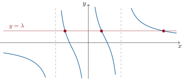
Deduce that for every $\lambda > 0$ , the equation $F(x) = \lambda$ has exactly $r$ real solutions, one in each interval $\intoo{p_i}{p_{i+1}}$ and one beyond $p_r$ . (Such equations govern eigenvalue perturbations; the intermediate value theorem is used at High School level here and proved in Chapter 13.)

Solution

Solution of Exercise 9.12.

On each interval avoiding the poles, $F'(x) = -\sum_i \frac{c_i}{(x - p_i)^2} < 0$ : strictly decreasing. As $x \to \pm\infty$ , every brick tends to $0$ : $F \to 0$ , from above at $+\infty$ (all bricks positive there) and from below at $-\infty$ . As $x \to p_i^+$ , the brick $\frac{c_i}{x - p_i}$ blows up to $+\infty$ and the others stay bounded: $F \to +\infty$ ; likewise $F \to -\infty$ as $x \to p_i^-$ .
Fix $\lambda > 0$ . On $\intoo{-\infty}{p_1}$ : $F$ decreases from $0^-$ to $-\infty$ , so $F < 0 < \lambda$ : no solution. On each $\intoo{p_i}{p_{i+1}}$ ( $1 \leq i \leq r-1$ ): $F$ decreases from $+\infty$ to $-\infty$ , hence takes the value $\lambda$ exactly once (intermediate value property plus strict monotonicity). On $\intoo{p_r}{+\infty}$ : $F$ decreases from $+\infty$ to $0^+$ , again exactly one solution. Total: exactly $r$ solutions, interlaced with the poles.

9.5 Problem: Partial fractions as an engine

Problem 9.1

Partial fraction decomposition looks like bookkeeping; this problem shows it is an engine. Fed with the fraction $\frac1{X(X+1)\cdots(X+k)}$ , it telescopes whole families of sums in closed form; fed with $\frac1{X^n - 1}$ , it produces trigonometric identities such as

\sum_{k=1}^{n-1}\frac{1}{\sin^2\frac{k\pi}{n}} = \frac{n^2-1}{3} ;

and, pushed one step further, that identity squeezes out one of the most celebrated formulas in mathematics, Euler’s

\sum_{k=1}^{\infty}\frac1{k^2} = \frac{\pi^2}{6}

— here obtained with nothing beyond this chapter’s algebra and high-school trigonometry. Throughout, $\omega = \eu^{2\iu\pi/n}$ ; limits of sequences are used at High School level (Chapter 11 formalizes them).

Part I — The telescope.

Decompose $\frac1{X(X+1)}$ and compute $\sum_{n=1}^{N} \frac1{n(n+1)}$ exactly; conclude that the sum tends to $1$ .
Same for $\frac1{X(X+2)}$ : show $\sum_{n=1}^{N} \frac1{n(n+2)} = \frac12\bigl(\frac32 - \frac1{N+1} - \frac1{N+2}\bigr) \to \frac34$ . (With a gap, two boundary terms survive at each end.)
Formalize the mechanism: if $F(X) = G(X) - G(X+1)$ for some rational $G$ without poles in $\intco1{+\infty}$ , then $\sum_{n=1}^N F(n) = G(1) - G(N+1)$ . Recover the value $\frac14$ of Exercise 9.8 by exhibiting the witness $G$ for $F = \frac1{X(X+1)(X+2)}$ .
Prove the general factorial telescope: for $k \geq 1$ ,

$\frac{1}{X(X+1)\cdots(X+k)} = \frac1k\biggl(\frac{1}{X(X+1)\cdots(X+k-1)} - \frac{1}{(X+1)\cdots(X+k)}\biggr),$

and deduce

$\sum_{n=1}^{\infty}\frac{1}{n(n+1)\cdots(n+k)} = \frac{1}{k \cdot k!} .$

Check the case $k = 2$ against question 3.
Evaluate the decomposition of Exercise 9.6 at well-chosen points to prove

$\sum_{j=0}^{n}(-1)^j\binom nj\,\frac1{j+1} = \frac1{n+1}, \qquad \sum_{j=0}^{n}(-1)^j\binom nj\,\frac1{j+2} = \frac1{(n+1)(n+2)} .$

Part II — The fraction $1/(X^n - 1)$ .

Show by the cover-up formula that

$\frac{1}{X^n - 1} = \frac1n\sum_{k=0}^{n-1}\frac{\omega^k}{X - \omega^k} .$
Two sanity checks: verify the formula directly for $n = 2$ , and show that the sum of the $n$ coefficients vanishes for $n \geq 2$ — explain why it must (consider $xF(x)$ as $x \to \infty$ ).
Re-derive by cover-up the identity of Exercise 9.7: $\frac{nX^{n-1}}{X^n-1} = \sum_k \frac1{X - \omega^k}$ .
Group conjugate poles to prove the real decomposition: with $\theta_k = \frac{2k\pi}n$ ,

$\frac{\omega^k}{X - \omega^k} + \frac{\omega^{n-k}}{X - \omega^{n-k}} = \frac{2\cos\theta_k\,X - 2} {X^2 - 2\cos\theta_k\,X + 1} ,$

and write down the full real decomposition of $\frac1{X^n-1}$ (distinguish $n$ odd and $n$ even).
Specialize to $n = 4$ and check against Exercise 9.4.

Part III — Trigonometric sums, and Euler’s $\pi^2/6$ . Let $P = 1 + X + \dots + X^{n-1}$ , whose roots are $\omega, \omega^2, \dots, \omega^{n-1}$ (all simple).

Using $\frac{P'}P = \sum_{k=1}^{n-1}\frac1{X - \omega^k}$ (Exercise 8.11), prove

$\sum_{k=1}^{n-1}\frac{1}{1 - \omega^k} = \frac{n-1}2 .$
Prove $\dfrac1{1 - \eu^{\iu\theta}} = \dfrac12 + \dfrac\iu2\,\frac{\cos(\theta/2)}{\sin(\theta/2)}$ for $\theta \notin 2\pi\Z$ (half-angle factorization, Method 3.11), and deduce from question 11 that $\sum_{k=1}^{n-1} \frac{\cos(k\pi/n)}{\sin(k\pi/n)} = 0$ — also visible by the symmetry $k \leftrightarrow n - k$ .
Differentiating the identity of question 11 (i.e. using $\bigl(\frac{P'}P\bigr)' = \frac{P''}P - \bigl(\frac{P'}P\bigr)^2$ evaluated at $X = 1$ ), prove

$\sum_{k=1}^{n-1}\frac{1}{(1 - \omega^k)^2} = \frac{(n-1)(5-n)}{12} .$
Writing $\cot t = \frac{\cos t}{\sin t}$ , deduce from questions 12–13 the two closed forms

$\sum_{k=1}^{n-1}\cot^2\frac{k\pi}n = \frac{(n-1)(n-2)}3, \qquad \sum_{k=1}^{n-1}\frac1{\sin^2\frac{k\pi}n} = \frac{n^2-1}3 .$
Verify both formulas by hand for $n = 3$ and $n = 4$ .
Prove the inequalities $\cot t < \frac1t < \frac1{\sin t}$ for $t \in \intoo0{\frac\pi2}$ (from $\sin t < t < \tan t$ ), and deduce, for $n = 2m + 1$ and $1 \leq k \leq m$ :

$\cot^2\frac{k\pi}n \;<\; \frac{n^2}{k^2\pi^2} \;<\; \frac1{\sin^2\frac{k\pi}n} .$
Sum these inequalities for $k = 1, \dots, m$ (using the symmetry $k \leftrightarrow n - k$ to halve the formulas of question 14) and squeeze:

$\sum_{k=1}^{\infty}\frac1{k^2} = \frac{\pi^2}6 .$

Part IV — Higher bricks.

By squaring the decomposition of $\frac1{X^2-1}$ and re-decomposing the cross term, prove

$\frac1{(X^2-1)^2} = \frac14\Bigl(\frac1{(X-1)^2} + \frac1{(X+1)^2}\Bigr) - \frac14\Bigl(\frac1{X-1} - \frac1{X+1}\Bigr),$

and check it at $X = 0$ .
Combine question 18, the telescope, and Euler’s value (question 17) to prove

$\sum_{n=2}^{\infty}\frac1{(n^2-1)^2} = \frac{\pi^2}{12} - \frac{11}{16} ,$

and confirm the value numerically to three decimals.
Differentiate the identity of question 8 to obtain a closed form for $\sum_{k=0}^{n-1}\frac1{(X - \omega^k)^2}$ , and check it at $X = 2$ , $n = 2$ .
Prove that for $k \geq 2$ ,

$\sum_{n=k}^{\infty}\frac{1}{\binom nk} = \frac{k}{k-1} .$

(Reduce to question 4 by writing $1/\binom nk$ with factorials.)
For $k = 3$ , give the exact partial sum $\sum_{n=3}^{N}\frac1{\binom n3}$ and its limit.

Part V — Synthesis.

As a capstone computation, write out the complete real decomposition of $\dfrac1{X^6 - 1}$ and check it at $X = 0$ .
Where exactly did the problem use: (i) the uniqueness of the decomposition; (ii) the roots of unity from Chapter 3; (iii) the logarithmic derivative from Exercise 8.11? One sentence each.
Synthesis, in a short paragraph: one algebraic identity — breaking a fraction into bricks — generated exact sums, trigonometric identities, and $\pi^2/6$ . Comment on the division of labor between algebra (exact decompositions, valid everywhere) and analysis (limits, squeezing), and point to where each thread is industrialized: telescoping and comparison in Chapter 17, integration of the bricks in Chapter 15.

Solution

Solution of Problem 9.1.

1. Cover-up: $\frac1{X(X+1)} = \frac1X - \frac1{X+1}$ . The sum telescopes:

\sum_{n=1}^{N}\Bigl(\frac1n - \frac1{n+1}\Bigr) = 1 - \frac1{N+1} \longrightarrow 1 .

2. $\frac1{X(X+2)} = \frac{1/2}X - \frac{1/2}{X+2}$ . Summing, the terms $\frac1n$ survive for $n = 1, 2$ and the terms $-\frac1{n+2}$ survive for $n = N-1, N$ :

\sum_{n=1}^{N}\frac1{n(n+2)} = \frac12\Bigl(1 + \frac12 - \frac1{N+1} - \frac1{N+2}\Bigr) \longrightarrow \frac34 .

3. If $F(X) = G(X) - G(X+1)$ , then $\sum_{n=1}^N F(n) = \sum_{n=1}^N\bigl(G(n) - G(n+1)\bigr) = G(1) - G(N+1)$ : all intermediate values cancel in pairs. For $F = \frac1{X(X+1)(X+2)}$ , the witness is $G(X) = \frac1{2X(X+1)}$ :

G(X) - G(X+1) = \frac{(X+2) - X}{2X(X+1)(X+2)} = F(X) ,

so $\sum_{n=1}^N F(n) = \frac14 - \frac1{2(N+1)(N+2)} \to \frac14$ , the value of Exercise 9.8.

4. Put the right-hand side over the common denominator $X(X+1)\cdots(X+k)$ :

\frac1k\cdot\frac{(X + k) - X}{X(X+1)\cdots(X+k)} = \frac{1}{X(X+1)\cdots(X+k)} ,

which is the identity. So $F_k(X) = \frac1k\bigl(G_k(X) - G_k(X+1)\bigr)$ with $G_k(X) = \frac1{X(X+1)\cdots(X+k-1)}$ , and question 3’s mechanism gives

\sum_{n=1}^{N}\frac1{n(n+1)\cdots(n+k)} = \frac1k\Bigl(\frac1{k!} - G_k(N+1)\Bigr) \longrightarrow \frac1{k\cdot k!} ,

since $G_k(1) = \frac1{k!}$ and $G_k(N+1) \to 0$ . For $k = 2$ : $\frac1{2\cdot2} = \frac14$ , matching question 3.

5. Exercise 9.6 gives $\frac{n!}{X(X+1)\cdots(X+n)} = \sum_{j=0}^n \frac{(-1)^j\binom nj}{X + j}$ . Evaluate at $X = 1$ : the left side is $\frac{n!}{(n+1)!} = \frac1{n+1}$ , the right side is $\sum_j(-1)^j\binom nj\frac1{1+j}$ : first identity. At $X = 2$ : the left side is $\frac{n!}{2\cdot3\cdots(n+2)} = \frac{n!\cdot1}{(n+2)!} = \frac1{(n+1)(n+2)}$ , the right side $\sum_j(-1)^j\binom nj\frac1{2+j}$ : second identity.

6. The poles $\omega^k$ are simple, and the simple-pole formula of Method 9.6 gives the coefficient

\frac{1}{\bigl(nX^{n-1}\bigr)_{X = \omega^k}} = \frac{1}{n\,\omega^{k(n-1)}} = \frac{\omega^k}{n\,\omega^{kn}} = \frac{\omega^k}n ,

using $\omega^{kn} = 1$ . Hence $\frac1{X^n-1} = \frac1n\sum_k \frac{\omega^k}{X - \omega^k}$ .

7. For $n = 2$ ( $\omega = -1$ ): $\frac12\bigl( \frac1{X-1} - \frac1{X+1}\bigr) = \frac12\cdot\frac{2}{X^2-1} = \frac1{X^2-1}$ : correct. The coefficients sum to $\frac1n\sum_k\omega^k = 0$ for $n \geq 2$ (Proposition 3.18). They must: $x\,F(x) \to \sum_k c_k$ as $x \to \infty$ for any decomposition with simple poles, while here $xF(x) = \frac{x}{x^n-1} \to 0$ since $n \geq 2$ .

8. Cover-up for $\frac{X^{n-1}}{X^n - 1}$ at $\omega^k$ : $\frac{A(\omega^k)}{B'(\omega^k)} = \frac{\omega^{k(n-1)}}{n\omega^{k(n-1)}} = \frac1n$ , so $\frac{X^{n-1}}{X^n-1} = \frac1n\sum_k\frac1{X - \omega^k}$ — the identity of Exercise 9.7 again.

9. With $c = \omega^k$ , $\conj c = \omega^{n-k}$ and $c\conj c = 1$ , $c + \conj c = 2\cos\theta_k$ :

\frac{c}{X - c} + \frac{\conj c}{X - \conj c} = \frac{c(X - \conj c) + \conj c(X - c)} {(X - c)(X - \conj c)} = \frac{2\cos\theta_k\,X - 2}{X^2 - 2\cos\theta_k\,X + 1} .

Grouping $k$ with $n - k$ in question 6: for odd $n$ ,

\frac1{X^n - 1} = \frac1n\Biggl(\frac1{X-1} + \sum_{k=1}^{(n-1)/2} \frac{2\cos\theta_k X - 2}{X^2 - 2\cos\theta_k X + 1}\Biggr) ;

for even $n$ , the extra self-paired pole $\omega^{n/2} = -1$ contributes $\frac{-1}{X+1}$ inside the parenthesis and the pair sum runs to $\frac n2 - 1$ .

10. $n = 4$ : $\theta_1 = \frac\pi2$ , $\cos\theta_1 = 0$ , so the pair term is $\frac{-2}{X^2+1}$ and

\frac1{X^4-1} = \frac14\Bigl(\frac1{X-1} - \frac1{X+1} - \frac2{X^2+1}\Bigr) ,

the decomposition of Exercise 9.4.

11. $P = \prod_{k=1}^{n-1}(X - \omega^k)$ (divide $X^n - 1$ by $X - 1$ ), so by Exercise 8.11, $\frac{P'}P = \sum_{k=1}^{n-1}\frac1{X-\omega^k}$ . At $X = 1$ : $P(1) = n$ and $P'(1) = \sum_{j=1}^{n-1}j = \frac{n(n-1)}2$ , whence

\sum_{k=1}^{n-1}\frac1{1 - \omega^k} = \frac{P'(1)}{P(1)} = \frac{n-1}2 .

12. Half-angle: $1 - \eu^{\iu\theta} = -2\iu\sin\frac\theta2\,\eu^{\iu\theta/2}$ , so

\frac1{1 - \eu^{\iu\theta}} = \frac{\eu^{-\iu\theta/2}}{-2\iu\sin\frac\theta2} = \frac{\iu\cos\frac\theta2 + \sin\frac\theta2} {2\sin\frac\theta2} = \frac12 + \frac\iu2\, \frac{\cos\frac\theta2}{\sin\frac\theta2} .

With $\theta = \theta_k = \frac{2k\pi}n$ : $\frac1{1-\omega^k} = \frac12 + \frac\iu2\cot\frac{k\pi}n$ . Summing over $k = 1, \dots, n-1$ and comparing with the real value $\frac{n-1}2$ of question 11: the real parts already account for everything, so $\sum_k\cot\frac{k\pi}n = 0$ — as the symmetry $\cot\frac{(n-k) \pi}n = -\cot\frac{k\pi}n$ also shows.

13. Differentiating $\frac{P'}P = \sum_k\frac1{X - \omega^k}$ :

\frac{P''}P - \Bigl(\frac{P'}P\Bigr)^2 = -\sum_{k=1}^{n-1}\frac1{(X - \omega^k)^2} .

At $X = 1$ : $P''(1) = \sum_{j=2}^{n-1}j(j-1) = 2\binom n3 = \frac{n(n-1)(n-2)}3$ (hockey-stick identity, or induction), so

\sum_{k=1}^{n-1}\frac1{(1 - \omega^k)^2} = \Bigl(\frac{n-1}2\Bigr)^2 - \frac{(n-1)(n-2)}3 = \frac{(n-1)\bigl(3(n-1) - 4(n-2)\bigr)}{12} = \frac{(n-1)(5-n)}{12} .

14. Squaring question 12’s formula, with $c_k = \cot\frac{k\pi}n$ :

\frac1{(1-\omega^k)^2} = \Bigl(\frac12 + \frac\iu2 c_k\Bigr)^2 = \frac14 - \frac{c_k^2}4 + \frac\iu2\,c_k .

Summing and using $\sum c_k = 0$ (question 12) and question 13: $\frac{n-1}4 - \frac14\sum_k c_k^2 = \frac{(n-1)(5-n)}{12}$ , so

\sum_{k=1}^{n-1}\cot^2\frac{k\pi}n = (n-1) - \frac{(n-1)(5-n)}3 = \frac{(n-1)(n-2)}3 .

Then $\frac1{\sin^2t} = 1 + \cot^2t$ gives $\sum_k\frac1{\sin^2\frac{k\pi}n} = (n-1) + \frac{(n-1)(n-2)}3 = \frac{n^2-1}3$ .

15. $n = 3$ : $\cot^2\frac\pi3 + \cot^2\frac{2\pi}3 = \frac13 + \frac13 = \frac23 = \frac{2\cdot1}3$ ; and $\frac1{\sin^2}$ sums to $\frac43 + \frac43 = \frac83 = \frac{9-1}3$ . $n = 4$ : $1 + 0 + 1 = 2 = \frac{3\cdot2}3$ ; and $2 + 1 + 2 = 5 = \frac{16-1}3$ . Both formulas check.

16. For $t \in \intoo0{\frac\pi2}$ , the classical comparison $\sin t < t < \tan t$ (area or convexity argument, familiar from High School) yields, taking reciprocals, $\cot t < \frac1t < \frac1{\sin t}$ , all three positive there; squaring preserves the order. With $t = \frac{k\pi}n$ , $1 \leq k \leq m$ , $n = 2m+1$ (so $t < \frac\pi2$ ):

\cot^2\frac{k\pi}n < \frac{n^2}{k^2\pi^2} < \frac1{\sin^2\frac{k\pi}n} .

17. By the symmetries $\cot^2\frac{(n-k)\pi}n = \cot^2\frac{k\pi}n$ and likewise for $\sin^2$ , question 14’s sums halve: $\sum_{k=1}^{m}\cot^2\frac{k\pi}n = \frac{(n-1)(n-2)}6 = \frac{m(2m-1)}3$ and $\sum_{k=1}^m\frac1{\sin^2\frac{k\pi}n} = \frac{n^2-1}6 = \frac{2m(m+1)}3$ . Summing question 16 over $k = 1, \dots, m$ and multiplying by $\frac{\pi^2}{n^2}$ :

\frac{\pi^2}{(2m+1)^2}\cdot\frac{m(2m-1)}3 \;<\; \sum_{k=1}^{m}\frac1{k^2} \;<\; \frac{\pi^2}{(2m+1)^2}\cdot\frac{2m(m+1)}3 .

Both bounds tend to $\frac{\pi^2}6$ as $m \to \infty$ (the ratios $\frac{m(2m-1)}{(2m+1)^2}$ and $\frac{2m(m+1)}{(2m+1)^2}$ both tend to $\frac12$ ), so by the squeeze the increasing partial sums converge and

\sum_{k=1}^{\infty}\frac1{k^2} = \frac{\pi^2}6 .

18. Square $\frac1{X^2-1} = \frac12\bigl(\frac1{X-1} - \frac1{X+1}\bigr)$ :

\frac1{(X^2-1)^2} = \frac14\Bigl(\frac1{(X-1)^2} + \frac1{(X+1)^2}\Bigr) - \frac12\cdot\frac1{(X-1)(X+1)} ,

and re-decompose the cross term $\frac1{(X-1)(X+1)} = \frac12\bigl(\frac1{X-1} - \frac1{X+1}\bigr)$ to get the stated form. At $X = 0$ : left side $1$ ; right side $\frac14(1 + 1) - \frac14(-1 - 1) = \frac12 + \frac12 = 1$ .

19. Sum question 18 over $n \geq 2$ . With $S = \sum_{k\geq1}\frac1{k^2} = \frac{\pi^2}6$ : $\sum_{n\geq2} \frac1{(n-1)^2} = S$ ; $\sum_{n\geq2}\frac1{(n+1)^2} = S - 1 - \frac14$ ; and the gap-two telescope $\sum_{n\geq2}\bigl( \frac1{n-1} - \frac1{n+1}\bigr) = 1 + \frac12 = \frac32$ . Hence

\sum_{n=2}^{\infty}\frac1{(n^2-1)^2} = \frac14\Bigl(2S - \frac54\Bigr) - \frac14\cdot\frac32 = \frac S2 - \frac{11}{16} = \frac{\pi^2}{12} - \frac{11}{16} \approx 0.135 .

Numerically: $\frac19 + \frac1{64} + \frac1{225} + \frac1{576} + \frac1{1225} + \dots \approx 0.1111 + 0.0156 + 0.0044 + 0.0017 + 0.0008 + \dots \approx 0.135$ : consistent.

20. Differentiate question 8’s identity $\sum_k\frac1{X-\omega^k} = \frac{nX^{n-1}}{X^n-1}$ :

\sum_{k=0}^{n-1}\frac1{(X - \omega^k)^2} = \frac{n^2X^{2n-2} - n(n-1)X^{n-2}(X^n - 1)}{(X^n - 1)^2} .

Check at $n = 2$ , $X = 2$ : right side $\frac{4\cdot4 - 2\cdot1\cdot3}{9} = \frac{10}9$ ; left side $\frac1{(2-1)^2} + \frac1{(2+1)^2} = 1 + \frac19 = \frac{10}9$ .

21. $\frac1{\binom nk} = \frac{k!\,(n-k)!}{n!} = \frac{k!}{(n-k+1)(n-k+2)\cdots n}$ , a product of $k$ consecutive integers downstairs. Substituting $j = n - k + 1$ (so $j$ runs over $\N^*$ as $n$ runs from $k$ ):

\sum_{n=k}^{\infty}\frac1{\binom nk} = k!\sum_{j=1}^{\infty}\frac1{j(j+1)\cdots(j+k-1)} = \frac{k!}{(k-1)\,(k-1)!} = \frac{k}{k-1} ,

by question 4 applied with $k - 1$ in place of $k$ (valid since $k - 1 \geq 1$ ).

22. For $k = 3$ : $\frac1{\binom n3} = \frac6{(n-2)(n-1)n}$ , so by question 3’s partial sum (shifted),

\sum_{n=3}^{N}\frac1{\binom n3} = 6\sum_{j=1}^{N-2}\frac1{j(j+1)(j+2)} = 6\Bigl(\frac14 - \frac1{2(N-1)N}\Bigr) = \frac32 - \frac3{(N-1)N} \longrightarrow \frac32 ,

the value $\frac k{k-1} = \frac32$ of question 21.

23. $n = 6$ : pairs $k = 1$ ( $\theta_1 = \frac\pi3$ , $2\cos\theta_1 = 1$ ) and $k = 2$ ( $\theta_2 = \frac{2\pi}3$ , $2\cos\theta_2 = -1$ ), plus the real poles $\pm1$ :

\frac1{X^6-1} = \frac16\Bigl(\frac1{X-1} - \frac1{X+1} + \frac{X - 2}{X^2 - X + 1} + \frac{-X - 2}{X^2 + X + 1}\Bigr) .

At $X = 0$ : left side $-1$ ; right side $\frac16(-1 - 1 - 2 - 2) = -1$ : correct.

24. (i) Uniqueness legitimizes every identification of coefficients — cover-up, the conjugate-pair grouping of question 9, and the differentiation tricks (questions 13, 20) all rest on it. (ii) Roots of unity supplied the poles of $X^n - 1$ , their symmetries ( $k \leftrightarrow n-k$ ), and the half-angle algebra of question 12 (Method 3.11). (iii) The logarithmic derivative $\frac{P'}P = \sum\frac{m_i}{X-a_i}$ converted information about the roots of $P = 1 + X + \dots + X^{n-1}$ into the numerical sums of questions 11 and 13 — the hinge between Parts II and III.

25. The decomposition is a purely algebraic identity, true for every value of the variable at once; that is what makes it an engine. Substituting integers and summing turned it into telescopes (Part I); substituting roots of unity and grouping conjugates turned it into trigonometric identities (Parts II and III); and only at the very last step did analysis enter — a squeeze between two closed forms — to deliver $\frac{\pi^2}6$ , a statement no finite substitution could reach. This division of labor (algebra produces exact finite identities, analysis passes to the limit) is the template for Chapter 17, where telescoping and comparison become systematic, and for Chapter 15, where each brick acquires a primitive and the same decompositions compute integrals instead of sums.

9.1 The field K(X)K(X)K(X)

9.2 Partial fraction decomposition over C\CC

9.3 Decomposition over R\RR

9.4 Exercises

9.5 Problem: Partial fractions as an engine

9.1 The field $K(X)$

9.2 Partial fraction decomposition over $\C$

9.3 Decomposition over $\R$