University Mathematics — Year 1 · Bachelor Year 1

24Plane Curves

The calculus of Chapters 14 and 16 was built for functions $y = f(x)$ ; most curves of geometry and mechanics — trajectories, circles rolled on circles, orbits — refuse that form and come instead as parametrized curves $t \mapsto (x(t), y(t))$ or as polar curves $r = r(\theta)$ . This classical chapter studies both, and closes with the conics.

24.1 Parametrized curves

Definition 24.1

A parametrized curve is a map $f \colon I \to \R^2$ , $t \mapsto M(t) = (x(t), y(t))$ , with $x, y$ of class $C^1$ (at least) on the interval $I$ . The velocity vector is $f'(t) = (x'(t), y'(t))$ ; the point $M(t_0)$ is regular when $f'(t_0) \neq (0,0)$ , and the tangent there is the line through $M(t_0)$ directed by $f'(t_0)$ .

Why $f'$ directs the tangent. By Taylor–Young componentwise, $M(t) = M(t_0) + (t - t_0) f'(t_0) + o(t - t_0)$ : the chord direction $\frac{M(t) - M(t_0)}{t - t_0}$ tends to $f'(t_0)$ . The regularity hypothesis is what makes the limit a direction: if $f'(t_0) = 0$ , the display collapses to $M(t) = M(t_0) + o(t - t_0)$ and says nothing about how the curve leaves the point — whence the separate treatment of singular points in the method below, where the first nonvanishing derivative takes over the role of $f'$ . Note also that the tangent line is a geometric object: any reparametrization changes $f'$ by a nonzero scalar factor and leaves the line unchanged. ∎

Method 24.2 (Studying a parametrized curve)

Reduce the domain using symmetries: relations between $M(-t)$ , $M(t + T)$ , … and $M(t)$ (reflections, translations, periodicity), then draw only the reduced part.
Variations: tabulate signs of $x'$ and $y'$ jointly; the curve moves right/left as $x'$ , up/down as $y'$ .
Remarkable points: horizontal tangent ( $y' = 0 \neq x'$ ), vertical tangent ( $x' = 0 \neq y'$ ); at a singular point ( $f' = 0$ ), examine higher derivatives for the tangent direction.
Asymptotic behavior at the ends of $I$ , then sketch.

Example 24.3 (Asymptotic branches, worked)

$x(t) = t$ , $y(t) = t + \dfrac1t$ on $\intoo{0}{+\infty}$ . As $t \to 0^{+}$ : $x \to 0$ while $y \to +\infty$ — the curve climbs along the vertical asymptote $x = 0$ (finite limit for one coordinate, infinite for the other). As $t \to +\infty$ : both coordinates blow up, so test a line: the difference

y(t) - x(t) = \frac1t \longrightarrow 0^{+}

exhibits the oblique asymptote $y = x$ , approached from above. In between, $y' = 1 - \frac1{t^2}$ vanishes at $t = 1$ : the point $(1, 2)$ is the low point of the branch, and $x' = 1 > 0$ throughout, so the curve always advances rightward. One arc, two asymptotes, one minimum: a complete picture from three computations — with the general recipe visible underneath: when $x, y \to \infty$ together, examine $y/x$ for a candidate slope (here $\to 1$ ), then $y - (\text{slope})\,x$ for the intercept and the side of approach.

Example 24.4 (The astroid)

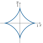
$x(t) = \cos^3 t$ , $y(t) = \sin^3 t$ . Symmetries: $M(t + 2\pi) = M(t)$ (study a period); $M(-t)$ is the reflection of $M(t)$ in the $x$ -axis; $M(\pi - t)$ in the $y$ -axis; $M(\frac\pi2 - t)$ in the diagonal $y = x$ : it suffices to study $t \in \intcc{0}{\frac\pi4}$ and unfold.

Velocity: $f'(t) = 3\sin t\cos t\,(-\cos t, \sin t)$ . On $\intoo{0}{\frac\pi2}$ all points are regular with tangent directed by $(-\cos t, \sin t)$ ; at $t = 0$ (the point $(1,0)$ ) the velocity vanishes: a cusp, where the curve reverses along the tangent direction $(-1, 0)\cdot(\pm)$ — by symmetry the four cusps sit at $(\pm1, 0), (0, \pm1)$ .

Example 24.5 (A figure-eight, studied in full)

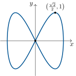
$x(t) = \sin t$ , $y(t) = \sin 2t$ (a Lissajous curve). Symmetries: $M(t + \pi) = (-x(t), y(t))$ (reflection in the $y$ -axis), $M(-t) = (-x(t), -y(t))$ (central symmetry), $M(\pi - t) = (x(t), -y(t))$ (reflection in the $x$ -axis): it suffices to study $t \in \intcc{0}{\frac\pi2}$ and unfold. Variations: $x' = \cos t \geq 0$ throughout, while $y' = 2\cos 2t$ is positive before $t = \frac\pi4$ and negative after: the arc climbs rightward to the summit $\bigl(\frac{\sqrt2}2,\ 1\bigr)$ at $t = \frac\pi4$ (horizontal tangent), then descends rightward to $(1, 0)$ at $t = \frac\pi2$ , where $x' = 0 \neq y'$ : vertical tangent. Double point: $M(0) = M(\pi) = (0,0)$ , with two different velocities

f'(0) = (1,\ 2), \qquad f'(\pi) = (-1,\ 2) :

two regular branches crossing at the origin at distinct angles — a double point, not a singular point: each passage is perfectly smooth, the two passages merely share their location. The whole curve is the figure-eight below.

The Lissajous curve ( t, 2t): a double point at the origin, where two regular branches cross with velocities (1, 2) and (-1, 2), and horizontal tangents at the four summits. Symmetry reduced all the work to a quarter-period. — The Lissajous curve $(\sin t, \sin 2t)$ : a double point at the origin, where two regular branches cross with velocities $(1, 2)$ and $(-1, 2)$ , and horizontal tangents at the four summits. Symmetry reduced all the work to a quarter-period.

The astroid ( 3 t, 3 t): four arcs meeting at four cusps. It is the curve traced by a point of a circle of radius 1/4 rolling inside the unit circle. — The astroid $(\cos^3 t, \sin^3 t)$ : four arcs meeting at four cusps. It is the curve traced by a point of a circle of radius $\frac14$ rolling inside the unit circle.

24.2 Polar curves

Definition 24.6

A polar curve is given by $r = r(\theta)$ : the point of parameter $\theta$ is

M(\theta) = r(\theta)\,\vec u(\theta), \qquad \vec u(\theta) = (\cos\theta, \sin\theta).

With $\vec v(\theta) = (-\sin\theta, \cos\theta) = \vec u\,'(\theta)$ , the velocity is

M'(\theta) = r'(\theta)\, \vec u(\theta) + r(\theta)\, \vec v(\theta) .

Consequences: where $r \neq 0$ , the point is regular, and the tangent makes with the ray the angle $V$ given by $\tan V = \frac{r}{r'}$ (angle between $M'$ and $\vec u$ ); where $r(\theta_0) = 0$ , the curve passes through the origin with tangent the ray $\theta = \theta_0$ (direction $\vec u(\theta_0)$ , read off $M'(\theta_0) = r'(\theta_0)\vec u(\theta_0)$ , or from the limit chord: the chord from $O$ to $M(\theta)$ is carried by $\vec u(\theta)$ itself, which tends to $\vec u(\theta_0)$ — so the rule holds even when $r'(\theta_0) = 0$ and the point is singular, which is why polar cusps at the origin, like the cardioid’s, get their tangent for free).

Example 24.7 (The cardioid)

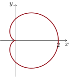
$r(\theta) = 1 + \cos\theta$ . Symmetry: $r(-\theta) = r(\theta)$ : reflection in the $x$ -axis; study $\theta \in \intcc{0}{\pi}$ . $r$ decreases from $2$ to $0$ ; at $\theta = \pi$ , $r = 0$ : the curve reaches the origin tangentially to the ray $\theta = \pi$ (the $x$ -axis), forming a cusp there — the heart’s point. Tangent at $\theta = 0$ : $r' = 0$ , so $\tan V = \infty$ : perpendicular to the axis.

The angle $V$ deserves one more reading. At $\theta = \frac\pi2$ : $r = 1$ and $r' = -1$ , so $\tan V = \frac{r}{r'} = -1$ : the tangent makes three-quarters of a right angle with the outgoing ray — the curve is already bending back toward its cusp. The formula $\tan V = r/r'$ delivers tangent directions along the whole curve with no computation of $M'(\theta)$ whatsoever: it is the polar analogue of reading a slope.

Example 24.8 (Polar to cartesian: a hidden circle)

What is the polar curve $r = 2\cos\theta$ ? Multiply by $r$ : $r^2 = 2r\cos\theta$ , i.e. $x^2 + y^2 = 2x$ , i.e.

(x - 1)^2 + y^2 = 1 :

the circle of center $(1, 0)$ and radius $1$ , passing through the origin. Bookkeeping matters: as $\theta$ runs over $\intoc{-\frac\pi2}{\frac\pi2}$ the whole circle is swept exactly once ( $r$ vanishes at both ends), and at $\theta = \pm\frac\pi2$ the rule “tangent at the origin along the ray $\theta = \theta_0$ ” gives a vertical tangent there — matching the geometry, since the vertical axis is indeed tangent to this circle at $O$ . For $\theta$ beyond that range, $r < 0$ retraces the same circle: a reminder that a polar curve is a parametrized object, allowed to pass over itself.

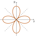
The four-petaled rose r = 2 (). The petals along the y-axis are traced with r < 0 (the point plots on the ray opposite to ); the dashed diagonals = ± π4 are the tangents at the origin, where r vanishes. — The four-petaled rose $r = \cos 2\theta$ (Exercise 24.4). The petals along the $y$ -axis are traced with $r < 0$ (the point plots on the ray opposite to $\theta$ ); the dashed diagonals $\theta = \pm\frac\pi4$ are the tangents at the origin, where $r$ vanishes.

The cardioid r = 1 +. Polar curves are read by sweeping the angle: the radius swells and shrinks as turns. — The cardioid $r = 1 + \cos\theta$ . Polar curves are read by sweeping the angle: the radius swells and shrinks as $\theta$ turns.

24.3 Arc length

Definition 24.9 (Length of an arc)

The length of a $C^1$ arc $f \colon \intcc{a}{b} \to \R^2$ is the integral of the speed:

L = \int_a^b \norm{f'(t)}\,\dd t = \int_a^b \sqrt{x'(t)^2 + y'(t)^2}\;\dd t .

(Motivation: on a small interval, $M(t + h) \approx M(t) + h f'(t)$ , so the arc is close to a polygon whose segment lengths sum to a Riemann sum of $\norm{f'}$ , Theorem 15.20.) For a polar curve $r = r(\theta)$ , the velocity $r'\vec u + r\vec v$ has orthogonal components, so

L = \int_{\theta_1}^{\theta_2} \sqrt{r'(\theta)^2 + r(\theta)^2}\;\dd\theta .

The length does not depend on the (monotone, $C^1$ ) parametrization chosen: substituting $t = \varphi(s)$ in the integral (Theorem 15.15) multiplies $f'$ by $\varphi'$ and $\dd t$ by $\varphi'^{-1}$ .

Example 24.10 (Sanity check: the circle)

For $f(t) = (R\cos t, R\sin t)$ on $\intcc{0}{2\pi}$ : $\norm{f'} = R$ , so $L = 2\pi R$ — the definition returns the circumference. Reparametrization test: the map $g(t) = (R\cos 2t, R\sin 2t)$ on $\intcc{0}{\pi}$ draws the same circle at doubled speed $\norm{g'} = 2R$ , and

\int_0^{\pi} 2R\,\dd t = 2\pi R

again: half the time, twice the speed, same length — the invariance promised in the definition, watched once on numbers. (Running $g$ on all of $\intcc{0}{2\pi}$ would give $4\pi R$ : a curve traversed twice is twice as long as a journey; length measures the parametrized path, and honest bookkeeping of the interval is part of the computation.) For the astroid $(\cos^3t, \sin^3t)$ : $\norm{f'} = 3\abs{\sin t\cos t} = \tfrac32\abs{\sin 2t}$ , and by symmetry $L = 4\int_0^{\pi/2} \tfrac32\sin 2t\,\dd t = 6$ : a curve drawn inside the unit circle, of length $6 < 2\pi$ . The weekend problem measures the most famous arch of all.

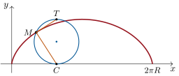
One arch of the cycloid (radius R = 1), the rolling circle at t = 2, and the two guide lines of the weekend problem: the chord MC to the contact point is normal to the curve, the chord MT to the top of the circle is tangent. — One arch of the cycloid (radius $R = 1$ ), the rolling circle at $t = 2$ , and the two guide lines of the weekend problem: the chord $MC$ to the contact point is *normal* to the curve, the chord $MT$ to the top of the circle is *tangent*.

24.4 Conics

Definition 24.11 (Focus–directrix definition)

Fix a point $F$ (focus), a line $D$ not through $F$ (directrix) and $e > 0$ (eccentricity). The conic of these data is

\mathcal{C} = \{M : d(M, F) = e\; d(M, D)\}:

an ellipse for $e < 1$ , a parabola for $e = 1$ , a hyperbola for $e > 1$ . (The circle appears as a degenerate limit $e \to 0$ .)

Example 24.12 (The definition, checked on a parabola)

Take the parabola $y^2 = 4x$ , i.e. $2p = 4$ : focus $F = (1, 0)$ and directrix $D : x = -1$ (the reduced form Theorem 24.13 puts them at $\pm\frac p2$ ). At the point $M = (1, 2)$ of the curve:

MF = \sqrt{(1-1)^2 + 2^2} = 2, \qquad d(M, D) = 1 - (-1) = 2 :

equal, as $e = 1$ demands. At $M' = (4, 4)$ : $MF' = \sqrt{9 + 16} = 5$ and $d(M', D) = 5$ again. The focus–directrix definition is not an abstraction: it is a pair of distances one can measure on any point, and the algebra of the reduced equations is nothing but this measurement done once and for all.

Theorem 24.13 (Reduced equations)

In a well-chosen orthonormal frame:

\text{ellipse: } \frac{x^2}{a^2} + \frac{y^2}{b^2} = 1 \quad (a \geq b > 0), \qquad \text{hyperbola: } \frac{x^2}{a^2} - \frac{y^2}{b^2} = 1, \qquad \text{parabola: } y^2 = 2px,

with, for the ellipse: foci at $(\pm c, 0)$ , $c = \sqrt{a^2 - b^2}$ , $e = \frac ca$ , and the bifocal characterization $MF + MF' = 2a$ ; for the hyperbola: $c = \sqrt{a^2 + b^2}$ , $e = \frac ca$ , $\abs{MF - MF'} = 2a$ , asymptotes $y = \pm\frac ba x$ .

Proof. Take the focus at the origin and the directrix vertical, $x = -h$ ( $h > 0$ ): the condition $MF^2 = e^2 d(M, D)^2$ reads $x^2 + y^2 = e^2 (x + h)^2$ . For $e = 1$ : $y^2 = 2hx + h^2$ , a parabola after the shift $x \mapsto x - \frac h2$ (so $p = h$ ). For $e \neq 1$ : completing the square in $x$ ,

(1 - e^2)\Bigl(x - \frac{e^2 h}{1 - e^2}\Bigr)^{\!2} + y^2 = e^2h^2 + \frac{e^4 h^2}{1 - e^2} = \frac{e^2 h^2}{1 - e^2} .

Set $X = x - \frac{e^2h}{1-e^2}$ (a shift of frame). When $e < 1$ , divide by the positive right-hand side: $\frac{X^2}{a^2} + \frac{y^2}{b^2} = 1$ with $a = \frac{eh}{1 - e^2}$ , $b = \frac{eh}{\sqrt{1-e^2}}$ ; when $e > 1$ , both sides of the display flip sign appropriately and the same division gives $\frac{X^2}{a^2} - \frac{y^2}{b^2} = 1$ with $a = \frac{eh}{e^2 - 1}$ , $b = \frac{eh}{\sqrt{e^2 - 1}}$ . The stated values of $c$ follow ( $c^2 = a^2 - b^2$ or $a^2 + b^2$ gives $c = ea$ in both cases, placing the focus correctly), and the bifocal properties are direct verifications on the reduced equations. In detail for the ellipse, with $F' = (c, 0)$ and $M = (X, y)$ on the curve:

MF'^2 = (X - c)^2 + y^2 = X^2 - 2cX + c^2 + b^2\Bigl(1 - \frac{X^2}{a^2}\Bigr) = \frac{c^2}{a^2}X^2 - 2cX + a^2 = (a - eX)^2 ,

using $c^2 + b^2 = a^2$ and $e = \frac ca$ ; since $\abs X \leq a$ and $e < 1$ , $a - eX > 0$ , so $MF' = a - eX$ with no square root ever extracted. The mirror computation gives $MF = a + eX$ , whence $MF + MF' = 2a$ , constant. For the hyperbola the same algebra yields $MF = \abs{a + eX}$ and $MF' = \abs{eX - a}$ , with difference $\pm2a$ according to the branch. ∎

Example 24.14

$\frac{x^2}{25} + \frac{y^2}{9} = 1$ : ellipse, $a = 5$ , $b = 3$ , $c = 4$ : foci $(\pm4, 0)$ , eccentricity $\frac45$ . Its parametrization: $(5\cos t, 3\sin t)$ — a circle stretched anisotropically; the sum of distances to the foci of any of its points is $10$ .

Example 24.15 (Reading an orbit from its polar equation)

The polar conic $r = \dfrac{1}{1 + \frac12\cos\theta}$ (Exercise 24.7 with $p = 1$ , $e = \frac12$ ) is an ellipse with a focus at the origin — the geometry of a planetary orbit with the sun at $O$ . Extract everything from $p$ and $e$ : from the reduction of Theorem 24.13, $a = \dfrac{p}{1 - e^2} = \dfrac{1}{3/4} = \dfrac43$ and $c = ea = \dfrac23$ . The two apsides check it with no theory at all:

r(0) = \frac{1}{3/2} = \frac23 = a - c \quad (\text{perihelion}), \qquad r(\pi) = \frac{1}{1/2} = 2 = a + c \quad (\text{aphelion}),

and their sum $\frac23 + 2 = \frac83 = 2a$ recovers the major axis. The polar form is the natural one whenever a focus is physically distinguished; the reduced cartesian form, whenever the symmetry axes are. Converting between the two is exactly what the completed-square computation of the theorem does.

Eccentricity as a dial, finally: keep $p = 1$ and turn $e$ in $r = \frac{1}{1 + e\cos\theta}$ . At $e = 0$ : the circle $r = 1$ . At $e = \frac12$ : the ellipse just studied, $r$ oscillating between $\frac23$ and $2$ . At $e = 1$ : $r(\theta) \to \infty$ as $\theta \to \pi$ — the curve no longer closes: a parabola, its farthest point pushed to infinity. At $e = 2$ : the denominator vanishes at $\cos\theta = -\frac12$ , and only $\theta \in \intoo{-\frac{2\pi}3}{\frac{2\pi}3}$ survives: one branch of a hyperbola, escaping along two asymptotic directions. One formula, the entire conic family, and the transition points $e = 1$ visible as the moment the denominator first reaches zero.

Remark 24.16 (Common pitfalls)

Double points are not singular points: at a self-crossing, each branch is regular; “singular” refers to $f'(t_0) = 0$ for one value of the parameter (Example 24.5 vs the astroid’s cusps). Vertical tangent versus cusp: $x'(t_0) = 0 \neq y'(t_0)$ is a regular point with vertical tangent; only $x' = y' = 0$ demands the higher-order expansion. Negative radii plot on the opposite ray: for $r(\theta) < 0$ the point is $-\abs{r}\,\vec u(\theta)$ , at angle $\theta + \pi$ (Exercise 24.5); forgetting this loses inner loops or doubles curves. Arc length integrates $\norm{f'}$ , not $f'$ : split the integral at the zeros of the speed — for the astroid, integrating $\frac32\sin 2t$ over a full period without absolute values gives $0$ , not $6$ . Conics must be reduced before being read: in $9x^2 + 25y^2 - 36x - 50y - 164 = 0$ , neither the axes, nor the center, nor the eccentricity is visible until the squares are completed (Exercise 24.6); and a vanishing quadratic part on one variable means parabola, not “degenerate ellipse”.

Remark 24.17 (Where these curves go)

Parametrized curves are the language of mechanics: trajectories are curves, velocity vectors are tangent vectors, and the arc length of Definition 24.9 is the distance run. The conics reappear wherever an inverse-square law acts — planetary orbits are ellipses with the sun at a focus. In Chapter 25, curves become the level sets of functions of two variables, and the tangent of this chapter meets the gradient of the next. The Year 2 volume adds curvature and the local canonical form of a curve; the weekend problem below already extracts, with this year’s tools only, everything the seventeenth century knew about its most celebrated curve.

Remark 24.18 (Perspectives inside Book 3)

This chapter consumes the whole first half of the volume and feeds the last chapter. Consumed: tangent vectors are derivatives (Chapter 14), arc length and areas are integrals (Chapter 15), cusps are settled by Taylor expansions (Chapter 16), the tautochrone is a linear differential equation (Chapter 5), and every distance and angle is Euclidean (Chapter 23). Fed: in Chapter 25, a curve $t \mapsto (x(t), y(t))$ drawn inside a level set $\{f = c\}$ is differentiated by the chain rule, and the resulting identity $\langle \nabla f,\ f'(t)\rangle = 0$ marries this chapter’s tangent vectors to the next one’s gradients — the tangent line of the curve and the normal direction of the surface are the same computation seen from both banks.

24.5 Exercises

Exercise 24.1 ★

Study and sketch the curve $x(t) = t^2$ , $y(t) = t^3$ (symmetries, variations, behavior at the singular point $t = 0$ ).

Solution

Solution of Exercise 24.1.

$M(-t) = (t^2, -t^3)$ : reflection in the $x$ -axis; study $t \geq 0$ . Both $x' = 2t$ and $y' = 3t^2$ are $\geq 0$ : the branch moves right and up, from $(0,0)$ to infinity. At $t = 0$ the velocity vanishes; expansions $x = t^2$ , $y = t^3$ show the tangent is the $x$ -axis ( $y/x = t \to 0$ ) with $y$ changing sign while $x \geq 0$ : a cusp pointing left. The curve is the semi-cubical parabola $y^2 = x^3$ .

Exercise 24.2 ★

For the cycloid $x(t) = t - \sin t$ , $y(t) = 1 - \cos t$ (the trajectory of a point of a rolling wheel of radius $1$ ): identify the period-translation symmetry, the singular points, and the tangent direction at $t = 0$ (expand $x$ and $y$ to the first nonzero orders).

Solution

Solution of Exercise 24.2.

$M(t + 2\pi) = M(t) + (2\pi, 0)$ : the curve repeats, translated by one wheel circumference; study one period. $x'(t) = 1 - \cos t \geq 0$ , $y'(t) = \sin t$ : the arch rises on $\intoo{0}{\pi}$ , falls on $\intoo{\pi}{2\pi}$ , culminating at $(\pi, 2)$ . Singular points where $x' = y' = 0$ : $t \in 2\pi\Z$ , on the ground. Near $t = 0$ :

x(t) = \frac{t^3}{6} + o(t^3), \qquad y(t) = \frac{t^2}{2} + o(t^2):

$x$ changes sign, $y \geq 0$ , and $\frac{x}{y^{3/2}}$ bounded: the tangent is vertical (direction $(0,1)$ ), a cusp where the tracked point momentarily has zero speed — the physical signature of rolling without slipping.

Exercise 24.3 ★

Give the tangent line to the curve $(\cos^3 t, \sin^3 t)$ at $t = \frac\pi4$ , and check that the segment of this tangent cut by the axes has length $1$ — a famous property of the astroid (true at every regular point).

Solution

Solution of Exercise 24.3.

At $t = \frac\pi4$ : $M = \bigl(\frac{\sqrt2}{4}, \frac{\sqrt2}{4}\bigr)$ , tangent direction $(-\cos t, \sin t) = \frac{1}{\sqrt2}(-1, 1)$ (Example 24.4). Tangent line: $y - \frac{\sqrt2}{4} = -(x - \frac{\sqrt2}{4})$ , i.e. $x + y = \frac{\sqrt2}{2}$ . Intercepts: $\bigl(\frac{\sqrt2}{2}, 0\bigr)$ and $\bigl(0, \frac{\sqrt2}{2}\bigr)$ ; the segment between them has length $\sqrt{\frac12 + \frac12} = 1$ .

(General point $t$ : the tangent at $(\cos^3 t, \sin^3 t)$ cuts the axes at $(\cos t, 0)$ and $(0, \sin t)$ — check that the line through these points has direction $(-\cos t, \sin t)$ and passes through $M(t)$ — and the cut segment has length $\sqrt{\cos^2 t + \sin^2 t} = 1$ .)

Exercise 24.4 ★

Sketch the polar curves $r = \cos 2\theta$ (four-petaled rose) and $r = \frac{1}{\cos\theta}$ on $\intoo{-\frac\pi2}{\frac\pi2}$ (recognize a line).

Solution

Solution of Exercise 24.4.

$r = \cos 2\theta$ : period $\pi$ in $\theta$ , symmetric in both axes; $r$ vanishes at $\theta = \pm\frac\pi4$ (tangents at the origin along the diagonals) and is negative for $\theta \in \intoo{\frac\pi4}{\frac{3\pi}{4}}$ , where the points plot on the opposite ray — producing four petals along the axes directions $\theta = 0, \frac\pi2, \pi, \frac{3\pi}{2}$ , each of maximal radius $1$ .

$r\cos\theta = 1$ is the equation $x = 1$ : the polar curve $r = \frac{1}{\cos\theta}$ is the vertical line $x = 1$ (swept once for $\theta \in \intoo{-\frac\pi2}{\frac\pi2}$ ).

Exercise 24.5 ★★

Study the polar curve $r = 1 + 2\cos\theta$ (a limaçon): domain where $r \geq 0$ vs $r < 0$ (points plotted with negative radius sit on the opposite ray), passage through the origin, inner loop, sketch.

Solution

Solution of Exercise 24.5.

$r(\theta) = 1 + 2\cos\theta$ vanishes for $\cos\theta = -\frac12$ : $\theta = \pm\frac{2\pi}{3}$ . Symmetry in the $x$ -axis; study $\theta \in \intcc{0}{\pi}$ . For $\theta \in \intco{0}{\frac{2\pi}{3}}$ : $r > 0$ , decreasing from $3$ to $0$ : outer arc, entering the origin tangent to the ray $\theta = \frac{2\pi}{3}$ . For $\theta \in \intoc{\frac{2\pi}{3}}{\pi}$ : $r < 0$ : the points $r\vec u(\theta)$ sit on the opposite ray (angle $\theta - \pi \in \intoc{-\frac\pi3}{0}$ ), with distance $\abs r$ growing from $0$ to $1$ : this draws a small inner loop through the origin. At $\theta = \pi$ , $r = -1$ and the point is $-\vec u(\pi) = (1, 0)$ : the loop closes on the positive $x$ -axis. Sketch: a big heart-like outer curve with maximum reach $3$ at $\theta = 0$ , plus a loop inside it through $O$ and $(1,0)$ .

Exercise 24.6 ★★

Identify the conic $9x^2 + 25y^2 - 36x - 50y - 164 = 0$ : reduce by completing squares, give center, semi-axes, foci, eccentricity.

Solution

Solution of Exercise 24.6.

Complete squares:

9(x^2 - 4x) + 25(y^2 - 2y) = 164 \iff 9(x-2)^2 + 25(y-1)^2 = 164 + 36 + 25 = 225 .

Dividing by $225$ : $\frac{(x-2)^2}{25} + \frac{(y-1)^2}{9} = 1$ : an ellipse of center $(2, 1)$ , semi-axes $a = 5$ (horizontal), $b = 3$ ; $c = \sqrt{25 - 9} = 4$ : foci $(2 \pm 4,\, 1) = (-2, 1)$ and $(6, 1)$ ; eccentricity $e = \frac45$ .

Exercise 24.7 ★★

Prove that the polar equation of a conic with focus at the origin is

r = \frac{p}{1 + e\cos\theta}

(directrix vertical at distance $\frac pe$ right of the focus). Which values of $\theta$ are allowed when $e > 1$ ?

Solution

Solution of Exercise 24.7.

Focus at the origin, directrix $D: x = d$ with $d = \frac pe > 0$ . For a point $M = (r\cos\theta, r\sin\theta)$ with $r > 0$ :

MF = r, \qquad d(M, D) = \abs{d - r\cos\theta},

and the conic condition $MF = e\,d(M, D)$ , in the regime where $M$ is on the focus side of the directrix ( $r\cos\theta < d$ ), reads $r = e(d - r\cos\theta)$ , i.e.

r(1 + e\cos\theta) = ed = p, \qquad r = \frac{p}{1 + e\cos\theta} .

For $e < 1$ the denominator never vanishes: all $\theta$ allowed (ellipse). For $e = 1$ : $\theta \neq \pi$ (parabola, open towards the directrix’s far side). For $e > 1$ : need $1 + e\cos\theta > 0$ , i.e. $\theta \in \intoo{-\theta_0}{\theta_0}$ with $\theta_0 = \arccos\bigl(-\frac1e\bigr)$ : one branch of the hyperbola (the other branch corresponds to the sign choice $r < 0$ , or to the second focus).

Exercise 24.8 ★★

From the bifocal property $MF + MF' = 2a$ , deduce the “gardener’s construction” of the ellipse, and prove that the tangent at $M$ makes equal angles with $MF$ and $MF'$ (reflection property; differentiate $\norm{M(t) - F} + \norm{M(t) - F'} = 2a$ and interpret the vanishing sum of unit-vector products).

Solution

Solution of Exercise 24.8.

Gardener: attach a string of length $2a$ to two stakes $F, F'$ and keep it taut with the tracing point $M$ : the constraint is exactly $MF + MF' = 2a$ , so the traced curve is the ellipse.

Reflection property: let $t \mapsto M(t)$ be a regular parametrization and $u(t) = \frac{M(t) - F}{\norm{M(t) - F}}$ , $u'(t)$ the analogous unit vector to $F'$ . Differentiating $\norm{M - F} + \norm{M - F'} = 2a$ , using $\frac{\dd}{\dd t}\norm{M - F} = \bigl\langle \frac{M - F}{\norm{M-F}},\, M'\bigr\rangle$ (chain rule on $\sqrt{\langle\cdot,\cdot\rangle}$ ):

\bigl\langle u + u',\, M'\bigr\rangle = 0 .

So the tangent direction $M'$ is orthogonal to the bisector direction $u + u'$ of the two focal rays: the tangent makes equal angles with $MF$ and $MF'$ . (A light ray from one focus reflects off the ellipse to the other focus.)

Exercise 24.9 ★★★

The lemniscate of Bernoulli is the polar curve $r^2 = \cos 2\theta$ (take $r = \sqrt{\cos2\theta}$ where defined).

Give its domain, symmetries, tangents at the origin, and sketch it.
Prove that it is the locus of points $M$ with $MF \cdot MF' = \frac12$ where $F, F' = \bigl(\pm\frac{1}{\sqrt2}, 0\bigr)$ . (Compute $MF^2\,MF'^2$ in polar coordinates.)

Solution

Solution of Exercise 24.9.

Domain: $\cos 2\theta \geq 0$ : $\theta \in \intcc{-\frac\pi4}{\frac\pi4} \cup \intcc{\frac{3\pi}{4}}{\frac{5\pi}{4}}$ . Symmetries: $\theta \mapsto -\theta$ ( $x$ -axis) and $\theta \mapsto \pi - \theta$ ( $y$ -axis): study $\intcc{0}{\frac\pi4}$ ; $r$ decreases from $1$ to $0$ . At $\theta = \pm\frac\pi4$ : $r = 0$ , tangents at the origin along the diagonals. The curve is the $\infty$ symbol: two symmetric loops meeting at $O$ , reaching $(\pm 1, 0)$ .
With $F, F' = (\pm c, 0)$ , $c = \frac{1}{\sqrt 2}$ , and $M = (r\cos\theta, r\sin\theta)$ :

$MF^2\, MF'^2 = \bigl((r\cos\theta - c)^2 + r^2\sin^2\theta\bigr) \bigl((r\cos\theta + c)^2 + r^2\sin^2\theta\bigr) = (r^2 + c^2)^2 - (2rc\cos\theta)^2 ,$

by the identity $(A - B)(A + B) = A^2 - B^2$ with $A = r^2 + c^2$ , $B = 2rc\cos\theta$ . With $c^2 = \frac12$ :

$MF^2 MF'^2 = \Bigl(r^2 + \frac12\Bigr)^2 - 2r^2\cos^2\theta = r^4 + r^2\bigl(1 - 2\cos^2\theta\bigr) + \frac14 = r^4 - r^2\cos 2\theta + \frac14 .$

On the lemniscate, $r^2 = \cos 2\theta$ : the first two terms cancel, leaving $MF^2MF'^2 = \frac14$ , i.e. $MF \cdot MF' = \frac12$ . Conversely, the computation read backwards shows the locus equation $MF\,MF' = \frac12$ is $r^2 = \cos 2\theta$ (for $r \neq 0$ ; and $O$ satisfies both).

Exercise 24.10 ★★

Compute the total length of the cardioid $r = 1 + \cos\theta$ using the polar formula of Definition 24.9 (the identity $1 + \cos\theta = 2\cos^2\frac\theta2$ turns the square root into $2\abs{\cos\frac\theta2}$ ).

Solution

Solution of Exercise 24.10.

$r = 1 + \cos\theta$ , $r' = -\sin\theta$ :

r^2 + r'^2 = 1 + 2\cos\theta + \cos^2\theta + \sin^2\theta = 2 + 2\cos\theta = 4\cos^2\frac\theta2 ,

so $\sqrt{r^2 + r'^2} = 2\abs{\cos\frac\theta2}$ and, by the symmetry in the $x$ -axis,

L = \int_0^{2\pi} 2\Bigl|\cos\frac\theta2\Bigr|\,\dd\theta = 2\int_0^{\pi} 2\cos\frac\theta2\,\dd\theta = 2\Bigl[4\sin\frac\theta2\Bigr]_0^{\pi} = 8 .

Another algebraic, $\pi$ -free perimeter.

Exercise 24.11 ★★

Show that the tangent to the ellipse $(a\cos t, b\sin t)$ at the point of parameter $t$ has equation

\frac{x\cos t}{a} + \frac{y\sin t}{b} = 1 ,

and deduce the tangent to $\frac{x^2}{a^2} + \frac{y^2}{b^2} = 1$ at a point $(x_0, y_0)$ of the ellipse: $\frac{x\,x_0}{a^2} + \frac{y\,y_0}{b^2} = 1$ (the “splitting of the squares” rule).

Solution

Solution of Exercise 24.11.

The point $(a\cos t, b\sin t)$ satisfies the equation: $\cos^2 t + \sin^2 t = 1$ . The line’s normal vector is $\bigl(\frac{\cos t}a, \frac{\sin t}b\bigr)$ , and its product with the velocity $(-a\sin t, b\cos t)$ is $-\sin t\cos t + \sin t\cos t = 0$ : the line passes through the point with the tangent direction — it is the tangent. For $(x_0, y_0)$ on the ellipse, write $\cos t = \frac{x_0}a$ , $\sin t = \frac{y_0}b$ and substitute:

\frac{x\,x_0}{a^2} + \frac{y\,y_0}{b^2} = 1 ,

obtained from the ellipse equation by “splitting” $x^2 \mapsto x\,x_0$ and $y^2 \mapsto y\,y_0$ .

Exercise 24.12 ★★★

The logarithmic spiral is the polar curve $r = \eu^{k\theta}$ ( $k > 0$ fixed, $\theta \in \R$ ).

Show that the angle $V$ between the radius and the tangent is constant ( $\tan V = \frac1k$ ) — the spiral crosses every ray at the same angle.
Show that rotating the spiral by an angle $c$ maps it onto its scaling by the factor $\eu^{-kc}$ : every rotation of the spiral is a magnification of it (self-similarity).
Compute the length of the arc $\theta \in \intoc{-\infty}{\theta_0}$ (as a limit of lengths on $\intcc{A}{\theta_0}$ , $A \to -\infty$ ) and observe that it is finite: a curve spiraling infinitely many times around the origin, of finite length.

Solution

Solution of Exercise 24.12.

$r' = k\eu^{k\theta}$ , so $\tan V = \frac{r}{r'} = \frac1k$ : constant. The spiral cuts every ray from the origin at the same angle $V = \arctan\frac1k$ .
In complex notation the spiral is $\{\eu^{k\theta} \eu^{\iu\theta} : \theta \in \R\}$ . Rotating by $c$ multiplies by $\eu^{\iu c}$ :

$\eu^{k\theta}\eu^{\iu(\theta + c)} = \eu^{-kc}\,\eu^{k(\theta + c)}\eu^{\iu(\theta+c)} ,$

and as $\theta + c$ runs over $\R$ this describes $\eu^{-kc}$ times the spiral: rotation $=$ scaling. No other smooth curve but lines and circles has this property.
$\sqrt{r^2 + r'^2} = \sqrt{1 + k^2}\,\eu^{k\theta}$ , so on $\intcc{A}{\theta_0}$ the length is $\frac{\sqrt{1+k^2}}{k}\bigl(\eu^{k\theta_0} - \eu^{kA}\bigr)$ , and as $A \to -\infty$ :

$L = \frac{\sqrt{1 + k^2}}{k}\,\eu^{k\theta_0} < \infty :$

infinitely many turns around the origin, finite total length (the turns shrink geometrically).

24.6 Problem: the cycloid, queen of curves

Problem 24.1

A wheel of radius $R$ rolls without slipping along the $x$ -axis; the point of the rim initially at the origin traces the cycloid. The seventeenth century fought over this curve — Galileo weighed paper cutouts of it, Wren measured it, Roberval computed its area, Huygens built clocks on it — and every one of their results is within reach of this chapter. We prove the four classics: the tangent construction, Wren’s length $8R$ , the area $3\pi R^2$ , and Huygens’ tautochrone property.

Part I — Rolling and the tangent.

After the wheel has turned by an angle $t$ , its center sits at $\Omega(t) = (Rt, R)$ (rolling without slipping: contact distance $=$ arc rolled). Show that the marked point is at

$M(t) = \bigl(R(t - \sin t),\; R(1 - \cos t)\bigr).$
Compute $f'(t)$ and show $\norm{f'(t)} = 2R\,\abs{\sin\frac t2}$ ; locate the singular points (cusps — cf. Exercise 24.2) and the top of each arch.
Let $C(t) = (Rt, 0)$ be the contact point and $T(t) = (Rt, 2R)$ the top of the wheel. Prove that for $0 < t < 2\pi$ the vector $M - C$ is normal to the curve at $M(t)$ and the vector $T - M$ is tangent: to draw the tangent to a cycloid, join the point to the top of its rolling circle. (Factor everything through $\sin\frac t2$ and $\cos\frac t2$ .)
Interpret question 3 kinematically: the contact point is the instantaneous center of rotation, and the speed of $M$ equals its distance to $C$ (for unit angular velocity). Verify $\norm{M - C} = 2R\abs{\sin\frac t2}$ .
Prove the height–speed relation

$\norm{f'(t)}^2 = 2R\,y(t) :$

on a cycloid traversed at unit angular velocity, the speed at each point is exactly the free-fall speed for a drop equal to the current height. (Keep this for Part IV.)

Part II — Wren’s theorem: the arch has length $8R$ .

Using Definition 24.9, compute the length of one arch:

$L = \int_0^{2\pi} 2R\sin\frac t2\,\dd t = 8R$

(Wren’s theorem, 1658). Four wheel diameters, and no $\pi$ anywhere.
Compute the arc length from the cusp: $s(t) = 4R\bigl(1 - \cos\frac t2\bigr)$ , and check $s(2\pi) = 8R$ .
Now measure the arc from the apex $t = \pi$ : $\sigma(t) = \abs{4R\cos\frac t2}$ . Prove the intrinsic relation

$\sigma^2 = 8R\,\bigl(2R - y\bigr) :$

the squared arc distance from the top is proportional to the height drop below the top.
Sanity checks: recover from question 8 that the half-arch from apex to cusp has length $4R$ , and compare with the astroid computation of Example 24.10 — both curves have algebraic, $\pi$ -free lengths; explain what makes this possible even though both are built from circles. (Look at the form of $\norm{f'}$ .)

Part III — Roberval’s area: $3\pi R^2$ .

Justify that the area between one arch and the ground is $A = \int_0^{2\pi} y(t)\,x'(t)\,\dd t$ (the substitution $x = x(t)$ in $\int y\,\dd x$ , Theorem 15.15; $x$ is increasing).
Compute

$A = R^2\int_0^{2\pi}(1 - \cos t)^2\,\dd t = 3\pi R^2 :$

exactly three times the area of the wheel — the ratio Galileo had guessed by weighing.
Same method for the astroid $(\cos^3t, \sin^3t)$ : show that the enclosed area is $\frac{3\pi}8$ (linearize $\sin^4 t\cos^2 t$ ; only the constant term survives over a full period).
Sanity check the formula of question 10 on the upper unit semicircle $(\cos t, \sin t)$ , $t$ from $\pi$ to $0$ : does it return $\frac\pi2$ ?

Part IV — Huygens’ tautochrone. Flip the arch: a frictionless bead slides, under gravity $g$ , inside the cycloidal bowl

x(t) = R(t + \sin t), \qquad y(t) = R(1 - \cos t) \qquad (t \in \intcc{-\pi}{\pi}),

whose lowest point is the origin ( $y$ measured upward).

Compute the speed $\norm{f'(t)} = 2R\cos\frac t2$ , the arc length from the bottom $s(t) = 4R\sin\frac t2$ , and prove the key identity

$y = \frac{s^2}{8R} .$
The bead released at rest from the point of parameter $t_0 > 0$ obeys energy conservation: if $s(\tau)$ denotes its arc position at time $\tau$ , then $\frac12\bigl( \frac{\dd s}{\dd\tau}\bigr)^2 + g\,y = g\,y_0$ . Rewrite this, using question 14, as

$\Bigl(\frac{\dd s}{\dd\tau}\Bigr)^{\!2} = \frac{g}{4R}\,\bigl(s_0^2 - s^2\bigr), \qquad s_0 = s(t_0).$
Differentiate with respect to $\tau$ and obtain the harmonic oscillator

$\frac{\dd^2 s}{\dd\tau^2} = -\frac{g}{4R}\,s ;$

solve it with Theorem 5.10 and the initial conditions: $s(\tau) = s_0\cos(\omega\tau)$ , $\omega = \sqrt{g/4R}$ .
Deduce the tautochrone property (Huygens, 1659): the time to reach the bottom,

$T_{\downarrow} = \frac{\pi}{2\omega} = \pi\sqrt{\frac Rg}\,,$

does not depend on the release point — beads released together from any two heights of the bowl arrive together.
Verify by substitution that $s(\tau) = s_0\cos\omega\tau$ satisfies the first-order energy equation of question 15 exactly (not only the differentiated one), and explain in one sentence why a circular pendulum is only approximately isochronous while the cycloid is exactly so.
Numerically: what radius $R$ makes the descent time exactly one second ( $g = 9.81$ )? Note how close the answer is to one meter, and how the full oscillation period $2\pi\sqrt{4R/g}$ compares with the small-angle pendulum formula $2\pi\sqrt{\ell/g}$ for $\ell = 4R$ .

Part V — Dividends, and synthesis.

Apply the tangent rule of question 3 at $t = \frac\pi2$ (take $R = 1$ ): compute $M$ , $T$ , the direction of $MT$ , and check it against $f'(\frac\pi2)$ .
(Trochoids) Mark instead a point at distance $d$ from the center ( $d \neq R$ ): the curve is $x = Rt - d\sin t$ , $y = R - d\cos t$ . Show that for $d < R$ the curve is regular everywhere and is the graph of no singular behavior ( $x' > 0$ : it advances), while for $d > R$ the abscissa $x'$ changes sign and the curve makes loops — the flanged railway wheel whose rim points travel backwards.
(Brachistochrone teaser) From the cusp $(\pi R, 2R)$ of the bowl to the bottom, compare the cycloid descent time $\pi\sqrt{R/g}$ with the time along the straight chute joining the same points (constant acceleration $g\sin\alpha$ along the chord): show the chord takes $\sqrt{\pi^2 + 4}\,\sqrt{R/g} \approx 3.72\sqrt{R/g}$ . The curve beats the line — it is, in fact, the fastest of all curves, a result of the calculus of variations.
Show that on the arch ( $0 < t < 2\pi$ ),

$\frac{\dd y}{\dd x} = \cot\frac t2, \qquad \frac{\dd^2 y}{\dd x^2} = -\frac{1}{4R\sin^4\frac t2} < 0 :$

the arch is concave, with vertical tangents exactly at the cusps.
Recover the vertical cusp tangent of Exercise 24.2 geometrically: compute the limit direction of the chord $MT$ of question 3 as $t \to 0^{+}$ , with no expansions at all.
Synthesis, in four sentences: which three named theorems this problem proved (with their numbers $8R$ , $3\pi R^2$ , $\pi\sqrt{R/g}$ and their authors); which single computational device ( $\sin\frac t2$ , $\cos\frac t2$ factorizations) powered all of Parts I, II and IV; how the intrinsic relation $y = s^2/8R$ converted geometry into a linear differential equation; and which chapter of this book each Part leaned on.

Solution

Solution of Problem 24.1.

1. Rolling without slipping means the contact point has traveled a distance equal to the arc of wheel unrolled: after turning by $t$ , the center is at $(Rt, R)$ . The marked point sits on the rim at angle $t$ behind the downward vertical (the wheel turns clockwise while advancing):

M(t) = \Omega(t) + R(-\sin t, -\cos t) = \bigl(R(t - \sin t),\ R(1 - \cos t)\bigr),

which is correct at $t = 0$ ( $M = (0,0)$ ) and at $t = \pi$ ( $M = (\pi R, 2R)$ , the top).

2. $f'(t) = R(1 - \cos t,\ \sin t)$ and

\norm{f'}^2 = R^2\bigl((1-\cos t)^2 + \sin^2 t\bigr) = 2R^2(1 - \cos t) = 4R^2\sin^2\frac t2 ,

so $\norm{f'} = 2R\abs{\sin\frac t2}$ . Singular points at $t \in 2\pi\Z$ : the cusps on the ground (Exercise 24.2); the top of the arch is $t = \pi$ , where the speed $2R$ is maximal.

3. Half-angle factorizations:

f'(t) = 2R\sin\frac t2\,\Bigl(\sin\frac t2,\ \cos\frac t2\Bigr), \quad M - C = 2R\sin\frac t2\,\Bigl(-\cos\frac t2,\ \sin\frac t2\Bigr),

T - M = \bigl(R\sin t,\ R(1 + \cos t)\bigr) = 2R\cos\frac t2\,\Bigl(\sin\frac t2,\ \cos\frac t2\Bigr).

For $0 < t < 2\pi$ , $\sin\frac t2 \neq 0$ : $M - C$ is orthogonal to the tangent direction $\bigl(\sin\frac t2, \cos\frac t2\bigr)$ (their product is $-\sin\frac t2\cos\frac t2 + \sin\frac t2\cos\frac t2 = 0$ ), and $T - M$ is parallel to it. The chord to the top of the wheel is the tangent; the chord to the contact point is the normal.

4. At each instant the wheel pivots about its contact point (that point has zero velocity: rolling without slipping), so every rigid point of the wheel moves orthogonally to the line joining it to $C$ , with speed (angular velocity $1$ ) equal to that distance. Check: $\norm{M - C} = 2R\abs{\sin\frac t2} = \norm{f'(t)}$ .

5. $2R\,y(t) = 2R\cdot 2R\sin^2\frac t2 = 4R^2\sin^2\frac t2 = \norm{f'(t)}^2$ . The speed at height $y$ is $\sqrt{2R\,y}$ — formally the law $v = \sqrt{2gh}$ of free fall, with the ground playing the ceiling; Part IV turns this observation into clockwork.

6. By Definition 24.9 and question 2 ( $\sin\frac t2 \geq 0$ on $\intcc{0}{2\pi}$ ):

L = \int_0^{2\pi} 2R\sin\frac t2\,\dd t = 2R\Bigl[-2\cos\frac t2\Bigr]_0^{2\pi} = 2R(2 + 2) = 8R .

Wren’s theorem: four diameters exactly.

7. $s(t) = \int_0^t 2R\sin\frac u2\,\dd u = 4R\bigl(1 - \cos\frac t2\bigr)$ ; $s(2\pi) = 4R(1+1) = 8R$ , consistent.

8. $\sigma(t) = \abs{s(t) - s(\pi)} = \abs{4R(1 - \cos\frac t2) - 4R} = 4R\abs{\cos\frac t2}$ , so $\sigma^2 = 16R^2\cos^2\frac t2$ ; and $2R - y = R(1 + \cos t) = 2R\cos^2\frac t2$ , whence $8R(2R - y) = 16R^2\cos^2\frac t2 = \sigma^2$ .

9. At the cusp $t = 0$ (or $2\pi$ ): $\sigma = 4R$ , half of $8R$ : the apex halves the arch. In both computations the speed is $\abs{\text{trigonometric polynomial in } t/2}$ , whose antiderivative is again trigonometric: the length is a difference of values of cosines — rational numbers times $R$ — with no arc of circle to measure, hence no $\pi$ . The circle itself has constant speed, so its length integral produces the full interval length $2\pi$ ; the cycloid’s speed vanishes at the ends and integrates algebraically.

10. The arch is swept with $x$ increasing from $0$ to $2\pi R$ ( $x' = R(1 - \cos t) \geq 0$ , vanishing only at isolated points). Substituting $x = x(t)$ in the area integral $\int_0^{2\pi R} y\,\dd x$ (Theorem 15.15) gives $A = \int_0^{2\pi} y(t)\,x'(t)\,\dd t$ .

11.

A = \int_0^{2\pi} R(1 - \cos t)\cdot R(1 - \cos t)\,\dd t = R^2\int_0^{2\pi}\bigl(1 - 2\cos t + \cos^2 t\bigr)\dd t = R^2\Bigl(2\pi - 0 + \pi\Bigr) = 3\pi R^2 ,

using $\int_0^{2\pi}\cos^2 = \pi$ . Exactly three wheel areas: Galileo’s balance said “about $3$ ”; Roberval’s computation says “exactly”.

12. With $x = \cos^3 t$ , $y = \sin^3 t$ : $y\,x' = -3\sin^4 t\cos^2 t$ . Linearize:

\sin^4 t\cos^2 t = \frac{1 - \cos 2t}{2}\cdot\frac{\sin^2 2t}{4} = \frac{\sin^2 2t}{8} - \frac{\sin^2 2t\cos 2t}{8} ,

and over $\intcc{0}{2\pi}$ : $\int\sin^2 2t = \pi$ , $\int \sin^2 2t\cos 2t = \bigl[\frac{\sin^3 2t}{6}\bigr] = 0$ . So $\oint y\,\dd x = -3\cdot\frac\pi8$ , and the enclosed area is $\frac{3\pi}8$ (the sign records the counterclockwise orientation).

13. For $(\cos t, \sin t)$ with $t$ from $\pi$ to $0$ , $x$ increases from $-1$ to $1$ and

\int_\pi^0 \sin t\cdot(-\sin t)\,\dd t = \int_0^\pi \sin^2 t\,\dd t = \frac\pi2 :

the formula returns the area of the upper half-disc, as it must.

14. $x' = R(1 + \cos t) = 2R\cos^2\frac t2$ , $y' = R\sin t = 2R\sin\frac t2\cos\frac t2$ , so $\norm{f'} = 2R\cos\frac t2$ (nonnegative on $\intcc{-\pi}{\pi}$ ). Arc from the bottom: $s(t) = \int_0^t 2R\cos\frac u2\,\dd u = 4R\sin\frac t2$ . Then

y = R(1 - \cos t) = 2R\sin^2\frac t2 = 2R\Bigl(\frac{s}{4R}\Bigr)^{\!2} = \frac{s^2}{8R} .

15. Energy conservation with $v = \frac{\dd s}{\dd\tau}$ and $y = \frac{s^2}{8R}$ , $y_0 = \frac{s_0^2}{8R}$ :

\Bigl(\frac{\dd s}{\dd\tau}\Bigr)^{\!2} = 2g(y_0 - y) = \frac{2g}{8R}\bigl(s_0^2 - s^2\bigr) = \frac{g}{4R}\bigl(s_0^2 - s^2\bigr).

16. Differentiating in $\tau$ : $2s's'' = -\frac{g}{4R}\,2ss'$ , so wherever $s' \neq 0$ (hence everywhere by continuity), $s'' = -\frac{g}{4R}s$ : the harmonic oscillator. By Theorem 5.10, $s(\tau) = A\cos\omega\tau + B\sin\omega\tau$ with $\omega = \sqrt{g/(4R)}$ ; the initial conditions $s(0) = s_0$ , $s'(0) = 0$ give $s(\tau) = s_0\cos\omega\tau$ .

17. The bead reaches the bottom when $s = 0$ , i.e. at $\omega\tau = \frac\pi2$ :

T_{\downarrow} = \frac{\pi}{2\omega} = \frac\pi2\sqrt{\frac{4R}{g}} = \pi\sqrt{\frac Rg}\,,

independent of $s_0$ : released from anywhere in the bowl, all beads arrive at the same instant — the tautochrone.

18. Substituting $s = s_0\cos\omega\tau$ : the left side is $s_0^2\omega^2\sin^2\omega\tau$ and the right side is $\frac{g}{4R}s_0^2(1 - \cos^2\omega\tau) = s_0^2\omega^2\sin^2\omega\tau$ : exact equality, so no spurious solution was introduced. For a circular arc, $y$ is not proportional to $s^2$ ( $y = \ell(1 - \cos\frac s\ell) = \frac{s^2}{2\ell} - \frac{s^4}{24\ell^3} + \dots$ ): the restoring term is only approximately linear, so the period of a circular pendulum drifts with amplitude, while the cycloid’s is rigorously constant.

19. $\pi\sqrt{R/g} = 1$ gives $R = \frac{g}{\pi^2} \approx \frac{9.81}{9.87} \approx 0.994$ m — almost exactly one meter. The full oscillation takes $\frac{2\pi}\omega = 2\pi\sqrt{4R/g}$ , which is precisely the small-angle formula $2\pi\sqrt{\ell/g}$ for a pendulum of length $\ell = 4R$ : Huygens suspended his pendulum from cycloidal cheeks of exactly that proportion.

20. At $t = \frac\pi2$ , $R = 1$ : $M = \bigl(\frac\pi2 - 1,\ 1\bigr)$ , $T = \bigl(\frac\pi2,\ 2\bigr)$ , so $T - M = (1, 1)$ . And $f'(\frac\pi2) = (1 - 0,\ 1) = (1, 1)$ : the chord to the top is the velocity, as promised.

21. For the trochoid, $x'(t) = R - d\cos t$ and $y'(t) = d\sin t$ . If $d < R$ : $x' \geq R - d > 0$ , the point always advances; the velocity never vanishes (its first component is positive): no singular point, a regular wave. If $d > R$ : $x'(0) = R - d < 0 < R + d = x'(\pi)$ , so the point moves backwards near the contact instants and forwards elsewhere: the curve crosses itself in loops. A point on the flange of a railway wheel (below the rail head, $d > R$ ) travels backwards at every turn.

22. The chord from the cusp $(\pi R, 2R)$ to the origin has length $L = R\sqrt{\pi^2 + 4}$ and slope angle $\alpha$ with $\sin\alpha = \frac{2R}{L}$ . Sliding from rest with constant acceleration $g\sin\alpha$ : $L = \frac12 g\sin\alpha\,T^2$ , so

T = \sqrt{\frac{2L}{g\sin\alpha}} = \sqrt{\frac{2L^2}{2Rg}} = \frac{L}{\sqrt{Rg}} = \sqrt{\pi^2 + 4}\,\sqrt{\frac Rg} \approx 3.72\sqrt{\frac Rg}\,,

against $\pi\sqrt{R/g} \approx 3.14\sqrt{R/g}$ for the cycloid: the curved path is faster. It is in fact the fastest possible — the brachistochrone — a theorem of the calculus of variations, beyond this volume.

23. $\dfrac{\dd y}{\dd x} = \dfrac{y'}{x'} = \dfrac{\sin t}{1 - \cos t} = \cot\dfrac t2$ (half-angle formulas). Then

\frac{\dd^2y}{\dd x^2} = \frac{\dd}{\dd t}\Bigl(\cot\frac t2\Bigr)\cdot\frac{1}{x'(t)} = -\frac{1}{2\sin^2\frac t2}\cdot\frac{1}{2R\sin^2\frac t2} = -\frac{1}{4R\sin^4\frac t2} < 0 :

concave throughout the arch; as $t \to 0^+$ or $2\pi^-$ the slope $\cot\frac t2 \to \pm\infty$ : vertical tangents at the cusps.

24. The chord direction is $T - M \parallel \bigl(\sin\frac t2, \cos\frac t2\bigr)$ , which tends to $(0, 1)$ as $t \to 0^{+}$ : the tangent at the cusp is vertical — recovered from pure geometry, with no Taylor expansion.

25. (i) Wren’s theorem, $L = 8R$ ; Roberval’s area, $A = 3\pi R^2$ (Galileo’s conjectured ratio $3$ ); Huygens’ tautochrone, $T_\downarrow = \pi\sqrt{R/g}$ . (ii) Every computation ran on the half-angle factorizations $f' = 2R\sin\frac t2(\sin\frac t2, \cos\frac t2)$ and their bowl analogue — one identity powering tangent, length and clock alike. (iii) The intrinsic relation $y = s^2/8R$ converted the energy equation into $s'' = -\frac{g}{4R}s$ , a linear equation with constant coefficients whose solutions are exactly isochronous. (iv) Part I used the differential calculus of Chapter 14, Part II–III the integral of Chapter 15, Part IV the differential equations of Chapter 5 — the cycloid is this book’s curriculum rolled into one curve.