University Mathematics — Year 1 · Bachelor Year 1

4Standard Functions

Analysis is only as useful as the stock of functions one masters. To the collection inherited from secondary school — powers, exponential, logarithm, trigonometric functions — this chapter adds their inverse functions ( $\arcsin$ , $\arccos$ , $\arctan$ ) and the hyperbolic family. Derivatives are used freely at High School level; the theory behind inverse functions is completed in Chapters 13 and 14.

4.1 Exponential, logarithm, powers

Proposition 4.1 (Recap and characterization)

$\exp \colon \R \to \intoo{0}{+\infty}$ and $\ln \colon \intoo{0}{+\infty} \to \R$ are reciprocal bijections, strictly increasing, with

\exp(x + y) = \exp x \exp y, \qquad \ln(xy) = \ln x + \ln y, \qquad \exp' = \exp, \qquad \ln'(x) = \frac 1x .

Moreover $\exp$ is the only differentiable function $f \colon \R \to \R$ with $f' = f$ and $f(0) = 1$ .

Proof. The recap is High School material. For uniqueness, let $f' = f$ , $f(0) = 1$ , and set $g(x) = f(x)\,\eu^{-x}$ . Then $g' = f'\eu^{-x} - f\eu^{-x} = 0$ , so $g$ is constant equal to $g(0) = 1$ : $f = \exp$ . ∎

Definition 4.2 (General powers)

For $x > 0$ and $\alpha \in \R$ : $\;x^\alpha = \eu^{\alpha \ln x}$ . For $a > 0$ , $a \neq 1$ , the logarithm to base $a$ is $\log_a x = \frac{\ln x}{\ln a}$ , the inverse of $x \mapsto a^x$ .

Example 4.3 (Solving exponential equations)

Solve $2^x = 5^{\,x-1}$ in $\R$ . Both sides are positive, so take logarithms — a reversible step:

x\ln2 = (x - 1)\ln5 \iff x(\ln2 - \ln5) = -\ln5 \iff x = \frac{\ln5}{\ln5 - \ln2} = \frac{\ln 5}{\ln\frac52} \approx 1.756 .

Next, solve $x^{\sqrt2} = 3$ for $x > 0$ : raise to the power $\frac1{\sqrt2}$ (i.e. apply the reciprocal bijection): $x = 3^{1/\sqrt2} = \eu^{(\ln 3)/\sqrt2} \approx 2.175$ . The insight: every equation mixing powers unwinds through $\ln$ and $\exp$ , because the definition $x^\alpha = \eu^{\alpha\ln x}$ reduces all power manipulations to arithmetic of exponents — but only on the domain $x > 0$ where that definition lives.

Example 4.4 (Doubling times)

A quantity grows by $3\%$ per step: after $n$ steps it is multiplied by $(1.03)^n$ . When does it double? Solve $(1.03)^n \geq 2$ :

n\ln(1.03) \geq \ln2 \iff n \geq \frac{\ln 2}{\ln 1.03} = \frac{0.6931}{0.02956} \approx 23.4 ,

so the first doubling occurs at step $24$ . (The financiers’ “rule of $72$ ”, which estimates the doubling time as $72$ divided by the rate in percent, is this computation with the approximation $\ln(1 + x) \approx x$ , quantified in Chapter 16.) Exponential processes are best reasoned about through their logarithms: on that scale, growth is linear and questions become divisions.

Example 4.5 (How long is $2^{2026}$ ?)

The number of decimal digits of an integer $N \geq 1$ is $\floor{\log_{10} N} + 1$ (indeed $N$ has $d$ digits exactly when $10^{d-1} \leq N < 10^d$ , i.e. $d - 1 \leq \log_{10}N < d$ ). For $N = 2^{2026}$ :

\log_{10} 2^{2026} = 2026\,\log_{10}2 = 2026 \times 0.301030 = 609.887 ,

so $2^{2026}$ has $610$ digits. The fractional part carries a bonus: $10^{0.887} \approx 7.7$ , so the number begins with $7$ . One multiplication answered a question about a number no one will ever write out — logarithms compress multiplicative size into additive size, which is their whole historical point (Example 7.12 makes that sentence precise).

Proposition 4.6 (Power rules and growth comparison)

For $x, y > 0$ and $\alpha, \beta \in \R$ :

x^{\alpha+\beta} = x^\alpha x^\beta, \quad (x^\alpha)^\beta = x^{\alpha\beta}, \quad (xy)^\alpha = x^\alpha y^\alpha, \quad (x^\alpha)' = \alpha\, x^{\alpha - 1}.

Growth scale as $x \to +\infty$ , for every $\alpha > 0$ and $\beta > 0$ :

\frac{(\ln x)^\beta}{x^\alpha} \longrightarrow 0, \qquad \frac{x^\alpha}{\eu^{\beta x}} \longrightarrow 0 .

Proof. The identities transcribe those of $\exp$ and $\ln$ through the definition. In detail for the second (the least obvious): $x^\alpha > 0$ and $\ln(x^\alpha) = \alpha\ln x$ (apply $\ln$ to the definition), so

(x^\alpha)^\beta = \eu^{\beta\ln(x^\alpha)} = \eu^{\beta\alpha\ln x} = x^{\alpha\beta} ;

the first and third are the same two-line unwindings via $\exp(u + v) = \exp u\exp v$ and $\ln(xy) = \ln x + \ln y$ . The derivative is the chain rule: $(\eu^{\alpha\ln x})' = \frac{\alpha}{x} \eu^{\alpha\ln x}$ .

Comparisons: from $\frac{\ln t}{t} \to 0$ (proved in the High School volume), substitute $t = x^{\alpha/\beta}$ : $\frac{\ln x}{x^{\alpha/\beta}} \to 0$ , then raise to the power $\beta$ . For the second, substitute $x = \ln u$ in the first. ∎

Example 4.7 (Two limits every reader should own)

What are $\lim_{x \to 0^+} x^x$ and $\lim_{x \to +\infty} x^{1/x}$ ? Both powers are defined through the exponential, so settle the exponent first:

x^x = \eu^{x\ln x}, \qquad x\ln x = -\frac{\ln(1/x)}{1/x} \longrightarrow 0 \quad (x \to 0^+), \qquad\text{so } x^x \longrightarrow \eu^0 = 1 ;

and $x^{1/x} = \eu^{(\ln x)/x} \to \eu^0 = 1$ as $x \to +\infty$ , directly by the growth comparison. The insight: an indeterminate power (of shape $0^0$ or $\infty^0$ ) is always handled by rewriting $u^v = \eu^{v\ln u}$ and analyzing the product $v \ln u$ — never by guessing from base and exponent separately. The function $x \mapsto \frac{\ln x}{x}$ that decided both limits is studied exhaustively in the weekend problem of this chapter.

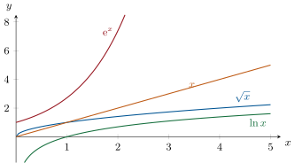
The growth scale of : near the right edge, x has barely passed 1.6 while x has left the frame. Every ratio (log over power, power over exponential) tends to 0 — the picture only hints at what the substitutions in the proof make exact. — The growth scale of Proposition 4.6: near the right edge, $\ln x$ has barely passed $1.6$ while $\eu^x$ has left the frame. Every ratio (log over power, power over exponential) tends to $0$ — the picture only hints at what the substitutions in the proof make exact.

Remark 4.8 (Common pitfalls with powers and logarithms)

Domains. $x^\alpha$ for irrational $\alpha$ needs $x > 0$ ; $(-8)^{1/3}$ is best avoided in favor of “the real cube root of $-8$ ”, because the rule $(x^\alpha)^\beta = x^{\alpha\beta}$ silently fails on negatives: $\bigl((-8)^2\bigr)^{1/6} = 2 \neq -2$ .
$\sqrt{x^2} = \abs x$ , not $x$ : forgetting the absolute value is the classic source of lost negative solutions.
$\ln(xy) = \ln x + \ln y$ requires $x, y > 0$ . For negative arguments, $\ln(xy)$ can be defined while the right-hand side is not.
Which function grows? In $x^\alpha$ the base varies; in $a^x$ the exponent does. Their growths are wildly different (Proposition 4.6), and hybrid expressions like $x^{\ln x}$ or $x^{1/x}$ must be rewritten as $\eu^{(\cdot)}$ before any reasoning — as in Example 4.7.

4.2 Inverse trigonometric functions

Definition 4.9 ( $\arcsin$ , $\arccos$ , $\arctan$ )

The restrictions

\sin \colon \intcc{-\tfrac\pi2}{\tfrac\pi2} \to \intcc{-1}{1}, \qquad \cos \colon \intcc{0}{\pi} \to \intcc{-1}{1}, \qquad \tan \colon \intoo{-\tfrac\pi2}{\tfrac\pi2} \to \R

are strictly monotonic bijections. Their inverse maps are written $\arcsin$ , $\arccos$ and $\arctan$ . Thus, for instance, $y = \arcsin x$ ( $x \in \intcc{-1}{1}$ ) is the angle in $\intcc{-\frac\pi2}{\frac\pi2}$ whose sine is $x$ .

From left to right: , , . Each inherits its graph from the restricted direct function by reflection in the line y = x. — From left to right: $\arcsin$ , $\arccos$ , $\arctan$ . Each inherits its graph from the restricted direct function by reflection in the line $y = x$ .

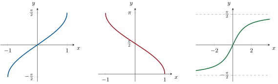
Proposition 4.10 (Derivatives)

On the interior of their domains:

\arcsin' x = \frac{1}{\sqrt{1 - x^2}}, \qquad \arccos' x = \frac{-1}{\sqrt{1 - x^2}}, \qquad \arctan' x = \frac{1}{1 + x^2}.

Proof. Anticipating the inverse-function rule proved in Chapter 14: if $f$ is a differentiable bijection and $f' \neq 0$ , then $(f^{-1})'(x) = \frac{1}{f'(f^{-1}(x))}$ . For $\arcsin$ : with $y = \arcsin x$ ,

\arcsin' x = \frac{1}{\cos y} = \frac{1}{\sqrt{1 - \sin^2 y}} = \frac{1}{\sqrt{1 - x^2}},

where $\cos y = +\sqrt{1 - \sin^2 y}$ because $y \in \intoo{-\frac\pi2}{\frac\pi2}$ forces $\cos y > 0$ . Similarly $\arccos' x = \frac{1}{-\sin y}$ with $\sin y > 0$ on $\intoo{0}{\pi}$ , and $\arctan' x = \frac{1}{1 + \tan^2 y} = \frac{1}{1 + x^2}$ using $\tan' = 1 + \tan^2$ . ∎

Example 4.11 (Recognizing a hidden constant)

Study $g(x) = \arctan\dfrac{1 - x}{1 + x}$ on $\intoo{-1} {+\infty}$ . Chain rule and a short computation:

g'(x) = \frac{1}{1 + \bigl(\frac{1-x}{1+x}\bigr)^2}\cdot \frac{-(1+x) - (1-x)}{(1+x)^2} = \frac{-2}{(1+x)^2 + (1-x)^2} = \frac{-1}{1 + x^2} ,

since $(1+x)^2 + (1-x)^2 = 2 + 2x^2$ . So $g' = -\arctan'$ : the function $g + \arctan$ has zero derivative on the interval $\intoo{-1}{+\infty}$ , hence is constant there; its value at $x = 0$ is $\arctan 1 + \arctan 0 = \frac\pi4$ . Conclusion:

\arctan\frac{1 - x}{1 + x} = \frac\pi4 - \arctan x \qquad (x > -1) .

On $\intoo{-\infty}{-1}$ the same derivative computation holds but the constant is different ( $-\frac{3\pi}4$ : evaluate the limit as $x \to -\infty$ ). The insight: “zero derivative implies constant” is an interval-by-interval statement — exactly the subtlety exploited in Exercise 4.6 and Exercise 4.10.

Proposition 4.12 (Standard identities)

For $x \in \intcc{-1}{1}$ : $\arcsin x + \arccos x = \dfrac{\pi}{2}$ .
For $x > 0$ : $\arctan x + \arctan\dfrac 1x = \dfrac{\pi}{2}$ (and $-\frac\pi2$ for $x < 0$ ).
$\sin(\arccos x) = \cos(\arcsin x) = \sqrt{1 - x^2}$ ; $\;\tan(\arcsin x) = \dfrac{x}{\sqrt{1 - x^2}}$ for $\abs x < 1$ .

Proof. (1) The derivative of $x \mapsto \arcsin x + \arccos x$ is zero on $\intoo{-1}{1}$ (Proposition 4.10), so the function is constant there, equal to its value $\frac\pi2$ at $0$ ; the endpoint values $\pm 1$ are checked directly ( $\frac\pi2 + 0$ and $-\frac\pi2 + \pi$ ).

(2) Same method on $\intoo{0}{+\infty}$ : the derivative is $\frac{1}{1+x^2} + \frac{-1/x^2}{1 + 1/x^2} = \frac{1}{1+x^2} - \frac{1}{x^2 + 1} = 0$ , and at $x = 1$ the sum is $2\arctan 1 = \frac\pi2$ . For $x < 0$ , use oddness of $\arctan$ .

(3) With $y = \arccos x \in \intcc{0}{\pi}$ : $\sin y \geq 0$ , so $\sin y = \sqrt{1 - \cos^2 y} = \sqrt{1 - x^2}$ ; likewise for $\cos(\arcsin x)$ , and the tangent formula is the quotient. ∎

Remark 4.13

$\arcsin(\sin\theta) = \theta$ holds only for $\theta \in \intcc{-\frac\pi2}{\frac\pi2}$ : for instance $\arcsin(\sin\pi) = 0 \neq \pi$ . The composition in the other direction, $\sin(\arcsin x) = x$ , is valid on all of $\intcc{-1}{1}$ .

Example 4.14 (Wrapping back to the principal interval)

Compute

\arctan\Bigl(\tan\frac{3\pi}4\Bigr) \qquad\text{and}\qquad \arctan\Bigl(\tan\frac{17\pi}5\Bigr).

The recipe: replace the angle by the unique angle of $\intoo{-\frac\pi2}{\frac\pi2}$ with the same tangent, i.e. subtract the right multiple of $\pi$ (the period of $\tan$ ). First: $\frac{3\pi}4 - \pi = -\frac\pi4$ , so the answer is $-\frac\pi4$ . Second: $\frac{17\pi} 5 - 3\pi = \frac{2\pi}5 \in \intoo{-\frac\pi2}{\frac\pi2}$ , so the answer is $\frac{2\pi}5$ . The computation is a Euclidean division of the angle by $\pi$ in disguise — and the analogous recipes for $\arcsin$ (reflect into $\intcc{-\frac\pi2}{\frac\pi2}$ , period $2\pi$ ) and $\arccos$ (reflect into $\intcc0\pi$ ) drive Exercise 4.1 and the piecewise answer of Exercise 4.10.

Example 4.15 (Adding arctangents safely)

Let us prove

\arctan\frac12 + \arctan\frac15 + \arctan\frac18 = \frac\pi4 .

Two ingredients: the tangent addition formula, and — the step beginners forget — a localization of the sum. First, $\tan(u + v) = \frac{\tan u + \tan v}{1 - \tan u\tan v}$ with $u = \arctan\frac12$ , $v = \arctan\frac15$ gives

\tan(u + v) = \frac{\frac12 + \frac15}{1 - \frac1{10}} = \frac{7/10}{9/10} = \frac79, \qquad\text{then}\qquad \tan\Bigl(u + v + \arctan\frac18\Bigr) = \frac{\frac79 + \frac18}{1 - \frac7{72}} = \frac{65/72}{65/72} = 1 .

Second, each of the three angles lies in $\intoo0{\frac\pi4}$ (their arguments are less than $1$ ), so the sum lies in $\intoo0{\frac{3\pi}4}$ ; the only angle there with tangent $1$ is $\frac\pi4$ . Without the localization the conclusion would be “ $\frac\pi4$ up to a multiple of $\pi$ ” — half a proof. The same two-step discipline runs Exercise 4.8 and Exercise 4.12.

Example 4.16 (An arctangent equation)

Solve $\arctan x + \arctan 2x = \dfrac\pi4$ . First localize: the left side has the sign of $x$ (both terms do), so any solution has $x > 0$ , and then the sum lies in $\intoo0\pi$ . Take tangents (injective on no interval of length $\pi$ , but combined with the localization this will suffice): the addition formula gives

\tan\bigl(\arctan x + \arctan 2x\bigr) = \frac{3x}{1 - 2x^2} = 1 \iff 2x^2 + 3x - 1 = 0 \iff x = \frac{-3 \pm \sqrt{17}}4 .

The negative root is discarded by the localization; for the positive candidate $x_0 = \frac{\sqrt{17} - 3}4 \approx 0.28$ , the sum lies in $\intoo0\pi$ with tangent $1$ , and the only such angle is $\frac\pi4$ (in $\intoo{\frac\pi2}\pi$ the tangent is negative): $x_0$ is the unique solution. Note the shape of the argument: taking tangents may create solutions, never lose them, so one solves the polynomial equation then filters by localization — the same forward-check discipline as squaring an equation.

4.3 Hyperbolic functions

Definition 4.17 ( $\cosh$ , $\sinh$ , $\tanh$ )

For $x \in \R$ :

\cosh x = \frac{\eu^x + \eu^{-x}}{2}, \qquad \sinh x = \frac{\eu^x - \eu^{-x}}{2}, \qquad \tanh x = \frac{\sinh x}{\cosh x}

(hyperbolic cosine, sine, tangent). $\cosh$ is even, $\sinh$ and $\tanh$ are odd.

Proposition 4.18 (Basic properties)

For all $x, y \in \R$ :

$\cosh^2 x - \sinh^2 x = 1$ ;
$\cosh' = \sinh$ , $\;\sinh' = \cosh$ , $\;\tanh' = 1 - \tanh^2 = \dfrac{1}{\cosh^2}$ ;
$\cosh(x+y) = \cosh x\cosh y + \sinh x \sinh y$ and $\sinh(x+y) = \sinh x \cosh y + \cosh x \sinh y$ ;
$\sinh$ is a strictly increasing bijection of $\R$ onto $\R$ ; $\cosh$ restricted to $\R_+$ is a strictly increasing bijection onto $\intco{1}{+\infty}$ ; $\tanh$ is a strictly increasing bijection of $\R$ onto $\intoo{-1}{1}$ .

Proof. (1) $\bigl(\frac{\eu^x + \eu^{-x}}{2}\bigr)^2 - \bigl(\frac{\eu^x - \eu^{-x}}{2}\bigr)^2 = \frac{(\eu^{2x} + 2 + \eu^{-2x}) - (\eu^{2x} - 2 + \eu^{-2x})}{4} = 1$ .

(2) Differentiate the defining formulas; for $\tanh$ , the quotient rule gives $\frac{\cosh^2 - \sinh^2}{\cosh^2}$ , which is both $1 - \tanh^2$ and $\frac{1}{\cosh^2}$ by (1).

(3) Expand the right-hand sides using the definitions. In detail for the first formula:

\cosh x\cosh y + \sinh x\sinh y = \frac{(\eu^x + \eu^{-x})(\eu^y + \eu^{-y}) + (\eu^x - \eu^{-x})(\eu^y - \eu^{-y})}{4} ;

of the eight products, the four “mixed” ones ( $\eu^{x-y}$ , $\eu^{y-x}$ ) cancel in pairs, while $\eu^{x+y}$ and $\eu^{-(x+y)}$ each appear twice: the total is $\frac{2\eu^{x+y} + 2\eu^{-(x+y)}}{4} = \cosh(x+y)$ . The sine formula is identical with the mixed terms surviving instead.

(4) $\sinh' = \cosh \geq 1 > 0$ , so $\sinh$ is strictly increasing, with limits $\pm\infty$ (dominant term $\pm\frac{\eu^{\abs x}}{2}$ ); the bijection statement then follows from the intermediate value theorem (used at High School level; systematic treatment in Chapter 13). On $\R_+$ , $\cosh' = \sinh \geq 0$ vanishing only at $0$ : strictly increasing from $\cosh 0 = 1$ to $+\infty$ . And $\tanh' > 0$ with limits $\pm 1$ at $\pm\infty$ : in detail,

\tanh x = \frac{\eu^x - \eu^{-x}}{\eu^x + \eu^{-x}} = \frac{1 - \eu^{-2x}}{1 + \eu^{-2x}} \xrightarrow[x \to +\infty]{} 1 ,

after dividing numerator and denominator by $\eu^x$ , and oddness gives the limit $-1$ at $-\infty$ ; the strictly increasing function $\tanh$ therefore maps $\R$ onto $\intoo{-1}1$ . ∎

Left: and , asymptotically glued to x/2 (dashed). Right: , increasing from -1 to 1. — Left: $\cosh$ and $\sinh$ , asymptotically glued to $\frac{\eu^x}{2}$ (dashed). Right: $\tanh$ , increasing from $-1$ to $1$ .

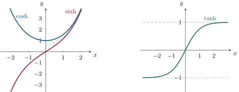
Remark 4.19 (Why “hyperbolic”?)

The point $(\cosh t, \sinh t)$ runs along the branch $x > 0$ of the hyperbola $x^2 - y^2 = 1$ (by Proposition 4.18 (1)), exactly as $(\cos t, \sin t)$ runs along the circle $x^2 + y^2 = 1$ . Every circular identity has a hyperbolic sibling, with sign changes governed by $\sinh^2 \leftrightarrow -\sin^2$ .

Example 4.20 (The addition formula for $\tanh$ )

Dividing the two addition formulas of Proposition 4.18 (3) by $\cosh x\cosh y$ :

\tanh(x + y) = \frac{\sinh x\cosh y + \cosh x\sinh y} {\cosh x\cosh y + \sinh x\sinh y} = \frac{\tanh x + \tanh y}{1 + \tanh x\,\tanh y} ,

the hyperbolic sibling of the tangent addition formula — with a $+$ where trigonometry has a $-$ . A dividend: since $\abs{\tanh} < 1$ , the right-hand side is a “velocity addition” rule that never leaves $\intoo{-1}1$ : if $u, v \in \intoo{-1}1$ then $\frac{u + v}{1 + uv} \in \intoo{-1}1$ as well (write $u = \tanh a$ , $v = \tanh b$ , possible by bijectivity, and read the formula backwards). Checking that algebraically, without hyperbolic functions, is a slightly painful exercise; parametrizing by $\tanh$ makes it one line — the same strategy that circular functions provide for the unit circle.

Proposition 4.21 (Inverse hyperbolic functions)

The inverses granted by Proposition 4.18 (4) have closed forms:

\operatorname{arsinh} x = \ln\bigl(x + \sqrt{x^2 + 1}\bigr) \ (x \in \R), \qquad \operatorname{arcosh} x = \ln\bigl(x + \sqrt{x^2 - 1}\bigr) \ (x \geq 1),

\operatorname{artanh} x = \frac 12 \ln\frac{1 + x}{1 - x} \ (\abs x < 1),

with derivatives $\frac{1}{\sqrt{x^2+1}}$ , $\frac{1}{\sqrt{x^2-1}}$ ( $x > 1$ ) and $\frac{1}{1 - x^2}$ respectively.

Proof. For $\operatorname{arsinh}$ : solve $x = \sinh y = \frac{\eu^y - \eu^{-y}}{2}$ . Setting $u = \eu^y > 0$ : $u^2 - 2xu - 1 = 0$ , so $u = x + \sqrt{x^2 + 1}$ (the root $x - \sqrt{x^2+1}$ is negative), and $y = \ln(x + \sqrt{x^2+1})$ . The other two are identical computations ( $u^2 - 2xu + 1 = 0$ for $\operatorname{arcosh}$ , keeping the root $\geq 1$ ; a two-line rearrangement for $\operatorname{artanh}$ ). Derivatives: differentiate the logarithmic expressions, e.g.

\bigl(\ln(x + \sqrt{x^2+1})\bigr)' = \frac{1 + \frac{x}{\sqrt{x^2+1}}}{x + \sqrt{x^2+1}} = \frac{1}{\sqrt{x^2 + 1}} . \qedhere

∎

Example 4.22 (Closed forms at work)

The solution of $\cosh t = 2$ with $t \geq 0$ is, by the closed form, $t = \operatorname{arcosh} 2 = \ln(2 + \sqrt3) \approx 1.317$ ; the other solution is $-t$ , by evenness — and indeed $\ln(2 - \sqrt3) = \ln\frac1{2 + \sqrt3} = -\ln(2 + \sqrt3)$ : the two roots $u = \eu^t$ of the quadratic $u^2 - 4u + 1 = 0$ are reciprocals, as their product $1$ (Vieta) demands. This tiny computation displays the general pattern: hyperbolic equations convert to quadratics in $\eu^t$ , and the symmetry $t \mapsto -t$ appears as the symmetry $u \mapsto 1/u$ of the quadratic — worth remembering when solving Exercise 4.7.

Method 4.23 (Choosing the right primitive form)

The three derivative patterns to memorize for integration (Chapter 15):

\int \frac{\dd x}{1 + x^2} = \arctan x + C, \qquad \int \frac{\dd x}{\sqrt{1 - x^2}} = \arcsin x + C, \qquad \int \frac{\dd x}{\sqrt{x^2 + 1}} = \operatorname{arsinh} x + C,

and for a general quadratic, reduce to these by completing the square and rescaling.

Remark 4.24 (Where this chapter is used)

This chapter is the working vocabulary of all the analysis to come. The growth scale of Proposition 4.6 decides convergence questions throughout Chapters 11 and 17; the derivative formulas of Proposition 4.10 and Proposition 4.21 are the primitives most often needed in Chapter 15, via Method 4.23; hyperbolic functions parametrize the solutions of the equation $y'' = y$ in Chapter 5 exactly as circular functions parametrize those of $y'' = -y$ . The characterization of $\exp$ by $f' = f$ , $f(0) = 1$ (Proposition 4.1) is the one-dimensional seed of the theory of linear differential equations, and the catenary curve $y = \cosh x$ returns among the plane curves of Chapter 24.

Remark 4.25 (Interlude: the inverse-function program)

This chapter ran one program four times: restrict a function until it becomes a strictly monotonic bijection, name the inverse, transport every formula through it. What was used at each step — that a continuous strictly monotonic function on an interval is a bijection onto an interval, and that its inverse is continuous, then differentiable away from critical points — was borrowed on High School credit. The debt is repaid inside this volume: Chapter 13 proves the bijection statement (the monotone inverse theorem, resting on the intermediate value theorem), and Chapter 14 proves the derivative rule $(f^{-1})' = 1/(f' \circ f^{-1})$ that silently produced every formula of Proposition 4.10 and Proposition 4.21. Reading those chapters with $\arcsin$ and $\operatorname{arsinh}$ in mind — as the worked examples the theory was built to justify — is the intended way around the apparent circularity.

4.4 Exercises

Exercise 4.1 ★

Compute without calculator: $\arcsin\frac{\sqrt 3}{2}$ ; $\;\arccos\bigl(-\frac 12\bigr)$ ; $\;\arctan(-1)$ ; $\;\arcsin\bigl(\sin\frac{5\pi}{6}\bigr)$ ; $\;\arccos\bigl(\cos\frac{7\pi}{4}\bigr)$ .

Solution

Solution of Exercise 4.1.

$\arcsin\frac{\sqrt 3}{2} = \frac\pi3$ ; $\;\arccos\bigl(-\frac12\bigr) = \frac{2\pi}{3}$ ; $\;\arctan(-1) = -\frac\pi4$ .

$\arcsin\bigl(\sin\frac{5\pi}{6}\bigr)$ : $\sin\frac{5\pi}{6} = \frac12$ , and the angle of $\intcc{-\frac\pi2}{\frac\pi2}$ with sine $\frac12$ is $\frac\pi6$ (not $\frac{5\pi}{6}$ ).

$\arccos\bigl(\cos\frac{7\pi}{4}\bigr)$ : $\cos\frac{7\pi}{4} = \frac{\sqrt 2}{2}$ , and the angle of $\intcc{0}{\pi}$ with that cosine is $\frac\pi4$ .

Exercise 4.2 ★

Give the domain of definition of $f(x) = \arcsin(2x - 1)$ and compute $f'$ where defined. Same questions for $g(x) = \arctan\sqrt{x}$ .

Solution

Solution of Exercise 4.2.

$f(x) = \arcsin(2x - 1)$ requires $-1 \leq 2x - 1 \leq 1$ , i.e. $x \in \intcc{0}{1}$ . On $\intoo{0}{1}$ , the chain rule and Proposition 4.10 give

f'(x) = \frac{2}{\sqrt{1 - (2x-1)^2}} = \frac{2}{\sqrt{4x - 4x^2}} = \frac{1}{\sqrt{x(1 - x)}} .

$g(x) = \arctan\sqrt x$ is defined for $x \geq 0$ , and for $x > 0$ :

g'(x) = \frac{1}{1 + x} \cdot \frac{1}{2\sqrt x} = \frac{1}{2\sqrt x\,(1 + x)} .

Exercise 4.3 ★

Prove that for all $x \in \R$ : $\cosh x + \sinh x = \eu^x$ and $(\cosh x + \sinh x)^n = \cosh nx + \sinh nx$ for every $n \in \Z$ (a hyperbolic de Moivre formula).

Solution

Solution of Exercise 4.3.

$\cosh x + \sinh x = \frac{\eu^x + \eu^{-x}}{2} + \frac{\eu^x - \eu^{-x}}{2} = \eu^x$ . Hence for $n \in \Z$ :

(\cosh x + \sinh x)^n = (\eu^x)^n = \eu^{nx} = \cosh nx + \sinh nx .

Exercise 4.4 ★

Simplify $\cos(2\arcsin x)$ and $\sin(2\arctan x)$ into algebraic expressions of $x$ .

Solution

Solution of Exercise 4.4.

With $y = \arcsin x$ : $\cos 2y = 1 - 2\sin^2 y = 1 - 2x^2$ , so $\cos(2\arcsin x) = 1 - 2x^2$ .

With $y = \arctan x$ : $\sin 2y = 2 \sin y \cos y = 2 \tan y \cos^2 y = \frac{2\tan y}{1 + \tan^2 y}$ , so $\sin(2\arctan x) = \dfrac{2x}{1 + x^2}$ .

Exercise 4.5 ★

Order, for large $x$ , the functions $x^{100}$ , $\;\eu^{\sqrt x}$ , $\;(\ln x)^{1000}$ , $\;\eu^{x/100}$ , $\;x^{\ln x}$ , from slowest to fastest growth, with justifications based on Proposition 4.6.

Solution

Solution of Exercise 4.5.

From slowest to fastest:

(\ln x)^{1000} \;\ll\; x^{100} \;\ll\; x^{\ln x} \;\ll\; \eu^{\sqrt x} \;\ll\; \eu^{x/100} .

Justifications: $(\ln x)^{1000}/x^{100} \to 0$ by Proposition 4.6 (logs lose to powers). $x^{100} = \eu^{100\ln x}$ and $x^{\ln x} = \eu^{(\ln x)^2}$ : since $(\ln x)^2 - 100\ln x \to +\infty$ , the second wins. $x^{\ln x} = \eu^{(\ln x)^2} \ll \eu^{\sqrt x}$ because $(\ln x)^2/\sqrt x \to 0$ (logs lose to the power $x^{1/4}$ , squared). Finally $\sqrt x - x/100 \to -\infty$ , so $\eu^{\sqrt x} \ll \eu^{x/100}$ .

Exercise 4.6 ★★

Study the function $f(x) = \arctan\dfrac{2x}{1 - x^2}$ on its domain: compute $f'$ , compare with $(2\arctan x)'$ , and express $f(x)$ in terms of $\arctan x$ on each of the three intervals of the domain.

Solution

Solution of Exercise 4.6.

Domain: $x \neq \pm 1$ , three intervals. On each,

f'(x) = \frac{\bigl(\frac{2x}{1-x^2}\bigr)'}{1 + \frac{4x^2}{(1-x^2)^2}} = \frac{\frac{2(1-x^2) + 4x^2}{(1-x^2)^2}} {\frac{(1-x^2)^2 + 4x^2}{(1-x^2)^2}} = \frac{2(1 + x^2)}{(1 + x^2)^2} = \frac{2}{1 + x^2} = (2\arctan x)' .

So $f(x) - 2\arctan x$ is constant on each interval. Values: at $x = 0$ , $f(0) = 0$ : the constant is $0$ on $\intoo{-1}{1}$ . As $x \to +\infty$ , $\frac{2x}{1-x^2} \to 0^-$ so $f \to 0$ , while $2\arctan x \to \pi$ : the constant is $-\pi$ on $\intoo{1}{+\infty}$ . By oddness, it is $+\pi$ on $\intoo{-\infty}{-1}$ . Summary: $f = 2\arctan x$ on $\intoo{-1}{1}$ , $f = 2\arctan x - \pi$ for $x > 1$ , $f = 2\arctan x + \pi$ for $x < -1$ . (This is the double-angle formula for the tangent, read through $\arctan$ .)

Exercise 4.7 ★★

Solve in $\R$ : $\;\cosh x = 2$ ; then $5\cosh x - 4 \sinh x = 3$ (express the solutions with logarithms). Hint for the second: write everything with $u = \eu^x$ .

Solution

Solution of Exercise 4.7.

$\cosh x = 2$ : with $u = \eu^x > 0$ , $u + u^{-1} = 4$ , so $u^2 - 4u + 1 = 0$ , $u = 2 \pm \sqrt 3$ : $x = \ln(2 + \sqrt 3)$ or $x = \ln(2 - \sqrt 3) = -\ln(2 + \sqrt 3)$ (the two solutions are opposite, as $\cosh$ is even; both are valid). Equivalently $x = \pm \operatorname{arcosh} 2$ .

$5\cosh x - 4\sinh x = 3$ : substituting the exponential definitions, $\frac{5(u + u^{-1}) - 4(u - u^{-1})}{2} = 3$ , i.e. $u + 9u^{-1} = 6$ , i.e. $u^2 - 6u + 9 = (u - 3)^2 = 0$ : $u = 3$ , one solution $x = \ln 3$ .

Exercise 4.8 ★★

Prove the identity $\arctan\frac{1}{2} + \arctan\frac{1}{3} = \frac{\pi}{4}$ , then Machin’s formula

4\arctan\frac 15 - \arctan\frac{1}{239} = \frac{\pi}{4}.

Hint: compute the tangent of both sides using the addition formula, and control in which interval each side lies.

Solution

Solution of Exercise 4.8.

Let $\alpha = \arctan\frac12 + \arctan\frac13$ . Addition formula:

\tan\alpha = \frac{\frac12 + \frac13}{1 - \frac12\cdot\frac13} = \frac{5/6}{5/6} = 1 .

Both arctangents lie in $\intoo{0}{\frac\pi4}$ (their arguments are in $\intoo{0}{1}$ ), so $\alpha \in \intoo{0}{\frac\pi2}$ ; the only angle there with tangent $1$ is $\frac\pi4$ .

Machin: let $\beta = \arctan\frac15$ . Double angle twice:

\tan 2\beta = \frac{2/5}{1 - 1/25} = \frac{5}{12}, \qquad \tan 4\beta = \frac{2 \cdot 5/12}{1 - 25/144} = \frac{120}{119}.

Then

\tan\Bigl(4\beta - \frac\pi4\Bigr) = \frac{\frac{120}{119} - 1}{1 + \frac{120}{119}} = \frac{1/119}{239/119} = \frac{1}{239}.

Location: $\beta < \arctan 1 = \frac\pi4$ and in fact $\tan 4\beta = \frac{120}{119}$ close to $1$ with $4\beta \in \intoo{0}{\frac\pi2}$ (since $\beta < \frac\pi8$ , as $\tan\frac\pi8 = \sqrt 2 - 1 > \frac15$ ); so $4\beta - \frac\pi4 \in \intoo{-\frac\pi4}{\frac\pi4}$ , where $\arctan$ inverts $\tan$ : $4\beta - \frac\pi4 = \arctan\frac{1}{239}$ , which is Machin’s formula.

Exercise 4.9 ★★

Prove that for all $x \geq 0$ : $\;x - \dfrac{x^3}{6} \leq \sin x \leq x$ (study the successive derivatives of the differences), and deduce $\lim_{x \to 0^+} \frac{x - \sin x}{x^3} = \frac 16$ is plausible — the limit itself is established in Chapter 16.

Solution

Solution of Exercise 4.9.

Let $f(x) = x - \sin x$ : $f(0) = 0$ and $f'(x) = 1 - \cos x \geq 0$ , so $f \geq 0$ on $\R_+$ : $\sin x \leq x$ .

Let $g(x) = \sin x - x + \frac{x^3}{6}$ : $g(0) = 0$ , $g'(x) = \cos x - 1 + \frac{x^2}{2}$ , $g'(0) = 0$ , $g''(x) = -\sin x + x = f(x) \geq 0$ on $\R_+$ . So $g'$ is increasing with $g'(0) = 0$ , hence $g' \geq 0$ , hence $g$ is increasing with $g(0) = 0$ : $g \geq 0$ , i.e. $x - \frac{x^3}{6} \leq \sin x$ on $\R_+$ .

Consequently $0 \leq \frac{x - \sin x}{x^3} \leq \frac 16$ for $x > 0$ : the ratio is trapped near $\frac16$ ’s scale, and Chapter 16 shows its limit is exactly $\frac 16$ .

Exercise 4.10 ★★★

For $x \in \intcc{-1}{1}$ , set $h(x) = \arcsin\bigl(2x\sqrt{1 - x^2}\,\bigr) - 2\arcsin x$ . One might expect $h = 0$ from the identity $\sin 2y = 2\sin y\cos y$ — but $h$ is not identically zero. Compute $h'$ on the open intervals where it exists, evaluate $h$ at well-chosen points, and give the full piecewise-constant description of $h$ on $\intcc{-1}{1}$ .

Solution

Solution of Exercise 4.10.

Write $y = \arcsin x$ , so $2x\sqrt{1 - x^2} = 2\sin y\cos y = \sin 2y$ and $h(x) = \arcsin(\sin 2y) - 2y$ .

For $\abs x \leq \frac{\sqrt 2}{2}$ : $2y \in \intcc{-\frac\pi2}{\frac\pi2}$ , so $\arcsin(\sin 2y) = 2y$ and $h = 0$ .

For $x \in \intoc{\frac{\sqrt 2}{2}}{1}$ : $2y \in \intoc{\frac\pi2}{\pi}$ , and the angle of $\intcc{-\frac\pi2}{\frac\pi2}$ with sine $\sin 2y$ is $\pi - 2y$ : so $h(x) = \pi - 4\arcsin x$ . (Check by derivative: there $h'(x) = \frac{2(1 - 2x^2)}{\abs{1 - 2x^2}\sqrt{1 - x^2}} - \frac{2}{\sqrt{1-x^2}} = \frac{-4}{\sqrt{1 - x^2}}$ , the derivative of $-4\arcsin x$ ; and at $x = 1$ , $h(1) = \arcsin 0 - 2\cdot\frac\pi2 = -\pi = \pi - 4\cdot\frac\pi2$ .)

For $x \in \intco{-1}{-\frac{\sqrt 2}{2}}$ , by oddness of $h$ : $h(x) = -\pi - 4\arcsin x$ .

Exercise 4.11 ★★★

(Gudermannian) Let $g(x) = \arctan(\sinh x)$ for $x \in \R$ . Prove that $g$ is an odd, strictly increasing bijection from $\R$ onto $\intoo{-\frac\pi2}{\frac\pi2}$ , that $g'(x) = \frac{1}{\cosh x}$ , and that $\tan g(x) = \sinh x$ , $\;\sin g(x) = \tanh x$ , $\;\cos g(x) = \frac{1}{\cosh x}$ : the function $g$ links circular and hyperbolic trigonometry without complex numbers.

Solution

Solution of Exercise 4.11.

$g = \arctan \circ \sinh$ is a composition of odd, strictly increasing functions, so it is odd and strictly increasing; as $x \to +\infty$ , $\sinh x \to +\infty$ so $g(x) \to \frac\pi2$ , and $g$ is a bijection onto $\intoo{-\frac\pi2}{\frac\pi2}$ (continuity plus the intermediate value theorem). Chain rule with Proposition 4.18 (1):

g'(x) = \frac{\cosh x}{1 + \sinh^2 x} = \frac{\cosh x}{\cosh^2 x} = \frac{1}{\cosh x} .

By construction $\tan g(x) = \sinh x$ . Then, since $g(x) \in \intoo{-\frac\pi2}{\frac\pi2}$ has positive cosine,

\begin{align*} \cos g(x) &= \frac{1}{\sqrt{1 + \tan^2 g(x)}} = \frac{1}{\sqrt{1 + \sinh^2 x}} = \frac{1}{\cosh x},\\ \sin g(x) &= \tan g(x) \cos g(x) = \frac{\sinh x}{\cosh x} = \tanh x . \end{align*}

Exercise 4.12 ★★

Prove that

\arctan 1 + \arctan 2 + \arctan 3 = \pi .

Hint: compute $\arctan 2 + \arctan 3$ first, localizing the sum as in Example 4.15; beware that the addition formula’s denominator is negative here.

Solution

Solution of Exercise 4.12.

Set $u = \arctan 2$ and $v = \arctan 3$ ; both lie in $\intoo{\frac\pi4}{\frac\pi2}$ (their arguments exceed $1$ ), so $u + v \in \intoo{\frac\pi2}{\pi}$ . The addition formula gives

\tan(u + v) = \frac{2 + 3}{1 - 6} = -1 ,

and the unique angle of $\intoo{\frac\pi2}{\pi}$ with tangent $-1$ is $\frac{3\pi}4$ : so $\arctan 2 + \arctan 3 = \frac{3\pi}4$ . (Blindly applying $\arctan$ to the tangent would give $-\frac\pi4$ , off by $\pi$ — the localization is what saves the computation, and the negative denominator $1 - 6$ is precisely the signal that the sum has left $\intoo{-\frac\pi2}{\frac\pi2}$ .) Adding $\arctan 1 = \frac\pi4$ :

\arctan 1 + \arctan 2 + \arctan 3 = \frac\pi4 + \frac{3\pi}4 = \pi .

4.5 Problem: The equation $x^y = y^x$

Problem 4.1

Which pairs of positive numbers satisfy $x^y = y^x$ ? Everyone knows one accidental-looking example, $2^4 = 4^2 = 16$ ; this problem shows that nothing about it is accidental. The whole equation is governed by the variations of the single function

f(t) = \frac{\ln t}{t} \qquad (t > 0),

whose study yields: the complete solution set (a diagonal plus one curved branch through $(\eu, \eu)$ ), a rational parametrization of the branch, the fact that $(2, 4)$ is its only integer point and the classification of all its rational points — plus, as dividends, the comparison of $\eu^\pi$ with $\pi^\eu$ and the monotone convergence of $\bigl(1 + \frac1n\bigr)^n$ to $\eu$ .

Part I — The function $f(t) = \ln t / t$ .

Justify that $f$ is differentiable on $\intoo0{+\infty}$ , compute $f'$ , and draw up the variation table: $f$ increases strictly on $\intoc0\eu$ , decreases strictly on $\intco\eu{+\infty}$ , with maximum $f(\eu) = \frac1\eu$ .
Determine the limits of $f$ at $0^+$ and $+\infty$ (Proposition 4.6), the sign of $f$ (negative on $\intoo01$ , zero at $1$ , positive beyond), and sketch the graph.
Check by direct computation that $f(2) = f(4)$ . (Keep this equality in mind: the entire problem grows out of it.)
Let $c \in \R$ . Discuss, according to the value of $c$ , the number of solutions of $f(t) = c$ : exactly one for $c \leq 0$ ; exactly two (one in $\intoo1\eu$ , one in $\intoo\eu{+\infty}$ ) for $0 < c < \frac1\eu$ ; exactly one for $c = \frac1\eu$ ; none for $c > \frac1\eu$ .
Deduce that $\eu^x > x^\eu$ for every $x > 0$ with $x \neq \eu$ , and in particular settle which of $\eu^\pi$ and $\pi^\eu$ is larger.

Part II — The equation and its curve. In this part $x, y > 0$ .

Show that $x^y = y^x \iff f(x) = f(y)$ .
Deduce the structure of the solution set: all diagonal pairs $(x, x)$ ; and the nontrivial pairs ( $x \neq y$ ), which satisfy: both coordinates are $> 1$ , and one lies in $\intoo1\eu$ while the other lies in $\intoo\eu{+\infty}$ .
Parametrize the nontrivial pairs: writing $y = tx$ with $t > 0$ , $t \neq 1$ , show that $x^y = y^x$ forces

$x(t) = t^{\frac1{t-1}}, \qquad y(t) = t\,x(t) = t^{\frac{t}{t-1}},$

and that conversely every such pair is a solution.
Verify that $t = 2$ gives $(2, 4)$ , and prove the symmetry $x(1/t) = y(t)$ , $y(1/t) = x(t)$ : inverting the parameter swaps the two coordinates.
Determine the limits of $x(t)$ and $y(t)$ as $t \to 1$ (both tend to $\eu$ ), as $t \to +\infty$ ( $x \to 1$ , $y \to +\infty$ ) and as $t \to 0^+$ ( $x \to +\infty$ , $y \to 1$ ). Describe the resulting branch: a curve asymptotic to the lines $x = 1$ and $y = 1$ , crossing the diagonal at $(\eu, \eu)$ .
Show that $t \mapsto x(t)$ is strictly decreasing on $\intoo1{+\infty}$ . (Study $h(t) = 1 - \frac1t - \ln t$ , whose sign controls the derivative of $\ln x(t) = \frac{\ln t}{t - 1}$ .)
Conclude that the nontrivial solutions define a strictly decreasing bijection $\varphi \colon \intoo1\eu \to \intoo\eu{+\infty}$ with $x^{\varphi(x)} = \varphi(x)^x$ , and that $\varphi$ is an involution of the branch: $\varphi(\varphi(x)) = x$ wherever both sides are defined.

Part III — Integer and rational points.

Prove that $(2, 4)$ and $(4, 2)$ are the only nontrivial integer solutions of $x^y = y^x$ .
For $n \in \N^*$ , apply the parametrization with $t = 1 + \frac1n$ and show that

$x_n = \Bigl(1 + \frac1n\Bigr)^{n}, \qquad y_n = \Bigl(1 + \frac1n\Bigr)^{n+1}$

is a nontrivial rational solution for every $n$ , with $(x_1, y_1) = (2, 4)$ .
Conversely, let $(x, y)$ be a nontrivial rational solution with $y > x$ , and write $t = y/x = 1 + \frac rs$ in lowest terms ( $r, s \in \N^*$ ). Using $x = t^{s/r}$ and admitting the uniqueness of prime factorization (familiar from school; proved in Chapter 6), show that $x$ rational forces both $s$ and $s + r$ to be $r$ -th powers of integers.
Show with the binomial theorem that $a^r - b^r = r$ has no integer solutions $a > b \geq 1$ when $r \geq 2$ , and conclude: the rational solutions of $x^y = y^x$ are exactly the pairs $(x_n, y_n)$ of question 14 (and their swaps).
Verify the case $n = 2$ numerically: compute $f(9/4)$ and $f(27/8)$ to four decimal places and check they agree.

Part IV — Dividends.

Use questions 7 and 11 to prove, with no further computation, that the sequence $x_n = \bigl(1 + \frac1n\bigr)^n$ is strictly increasing with $x_n < \eu$ , that $y_n = \bigl(1 + \frac1n\bigr)^{n+1}$ is strictly decreasing with $y_n > \eu$ , and that both converge to $\eu$ . (The parameter $t_n = 1 + \frac1n$ decreases to $1$ .)
Establish the general comparison rule for $1 < a < b$ : if $\eu \leq a$ then $a^b > b^a$ ; if $b \leq \eu$ then $a^b < b^a$ ; and show by the two examples $(2, 3)$ and $(2, 5)$ that in the mixed case $a < \eu < b$ both outcomes really occur.
Suppose the involution $\varphi$ of question 12 is differentiable at $\eu$ (it is). Differentiate the identity $\varphi(\varphi(x)) = x$ at $x = \eu$ and deduce $\varphi'(\eu) = -1$ : the branch crosses the diagonal at right angles to it.
Find the unique solution pair with $y = 3x$ , in closed form, and check it numerically to four decimals via $f$ .
Among the numbers $\sqrt2$ , $\sqrt[3]3$ , $\sqrt[4]4$ , $\sqrt[5]5$ , determine the largest and identify the two that are equal. (Compare $n^{1/n} = \eu^{f(n)}$ .)

Part V — Synthesis.

Describe the complete solution set of $x^y = y^x$ in the quarter-plane $x, y > 0$ — diagonal plus branch, their intersection $(\eu, \eu)$ , the asymptotes, the integer point $(2, 4)$ , the rational points accumulating at $(\eu, \eu)$ — in a form you could sketch from memory.
Where exactly did the problem use: (i) the growth comparisons of Proposition 4.6; (ii) the intermediate value theorem (through the bijection statements); (iii) the admitted uniqueness of prime factorization? One sentence each.
Moral, in a short paragraph: a single variation table solved an equation in two unknowns, classified its rational points, and proved the monotone convergence of $\bigl(1 + \frac1n\bigr)^n$ — comment on this economy, and name where each thread is industrialized later in the volume (Chapter 11 for the sequence, Chapter 14 for variation tables, Chapter 16 for the precision the table lacks).

Solution

Solution of Problem 4.1.

1. $f$ is a quotient of differentiable functions with nonvanishing denominator on $\intoo0{+\infty}$ , and

f'(t) = \frac{\frac1t \cdot t - \ln t}{t^2} = \frac{1 - \ln t}{t^2} ,

positive for $t < \eu$ , zero at $t = \eu$ , negative for $t > \eu$ : $f$ increases strictly on $\intoc0\eu$ , decreases strictly on $\intco\eu{+\infty}$ , with maximum $f(\eu) = \frac1\eu$ .

2. As $t \to 0^+$ : $\ln t \to -\infty$ and $\frac1t \to +\infty$ , so $f(t) \to -\infty$ . As $t \to +\infty$ : $f(t) \to 0$ by the growth comparison of Proposition 4.6 ( $\beta = \alpha = 1$ ). Sign: that of $\ln t$ , so $f < 0$ on $\intoo01$ , $f(1) = 0$ , $f > 0$ on $\intoo1{+\infty}$ . The graph climbs from $-\infty$ , crosses zero at $1$ , peaks at $(\eu, \frac1\eu)$ , then decays to $0^+$ .

3. $f(4) = \frac{\ln 4}4 = \frac{2\ln 2}4 = \frac{\ln 2}2 = f(2)$ .

4. By the variation table and the intermediate value theorem (used at High School level; formalized in Chapter 13). For $c < 0$ : solutions exist only where $f < 0$ , i.e. in $\intoo01$ where $f$ is a strictly increasing bijection onto $\intoo{-\infty}0$ : exactly one. For $c = 0$ : only $t = 1$ . For $0 < c < \frac1\eu$ : on $\intoo1\eu$ , $f$ increases from $0$ to $\frac1\eu$ : one solution; on $\intoo\eu{+\infty}$ , $f$ decreases from $\frac1\eu$ to $0$ : one more; total two. For $c = \frac1\eu$ : only the maximum point $t = \eu$ . For $c > \frac1\eu$ : none.

5. For $x \neq \eu$ , strict maximality gives $f(x) < f(\eu)$ , i.e. $\frac{\ln x}x < \frac1\eu$ , i.e. $\eu\ln x < x$ , i.e. $\ln(x^\eu) < \ln(\eu^x)$ : $x^\eu < \eu^x$ . With $x = \pi$ : $\eu^\pi > \pi^\eu$ (numerically $23.14 > 22.46$ ).

6. For $x, y > 0$ , both sides are positive, so

x^y = y^x \iff y\ln x = x\ln y \iff \frac{\ln x}x = \frac{\ln y}y \iff f(x) = f(y) ,

dividing by $xy > 0$ .

7. Let $f(x) = f(y) = c$ with $x \neq y$ . If $c \leq 0$ or $c = \frac1\eu$ , question 4 says the equation $f = c$ has a single solution: impossible. So $0 < c < \frac1\eu$ , and again by question 4 the two solutions are one point of $\intoo1\eu$ and one of $\intoo\eu{+\infty}$ : both coordinates exceed $1$ and they straddle $\eu$ .

8. Substituting $y = tx$ in $y\ln x = x\ln y$ :

tx\ln x = x(\ln t + \ln x) \iff (t - 1)\ln x = \ln t \iff \ln x = \frac{\ln t}{t - 1} ,

so $x = t^{1/(t-1)}$ and $y = tx = t^{1 + \frac1{t-1}} = t^{t/(t-1)}$ . Conversely, for these values, $\ln y = \frac{t\ln t}{t-1} = t\ln x$ and $y = tx$ , so $\frac{\ln y}y = \frac{t\ln x}{tx} = \frac{\ln x}x$ : a solution. Every nontrivial solution has some ratio $t = y/x \in \intoo0{+\infty} \setminus \{1\}$ , so the parametrization is complete.

9. $t = 2$ : $x = 2^{1/1} = 2$ , $y = 2^{2/1} = 4$ . And

x(1/t) = (1/t)^{\frac1{\frac1t - 1}} = (t^{-1})^{\frac{t}{1 - t}} = t^{\frac{t}{t - 1}} = y(t) ,

then $y(1/t) = \frac1t\,x(1/t) = \frac{y(t)}t = x(t)$ : the parameter change $t \mapsto 1/t$ swaps the coordinates, as the symmetry of the equation demands.

10. As $t \to 1$ : $\frac{\ln t}{t-1} \to 1$ (it is the difference quotient of $\ln$ at $1$ ), so $x \to \eu^1 = \eu$ and $y = tx \to \eu$ . As $t \to +\infty$ : $\ln x = \frac{\ln t}{t-1} \to 0$ so $x \to 1$ , while $\ln y = \frac{t\ln t}{t-1} \to +\infty$ so $y \to +\infty$ . As $t \to 0^+$ : $\ln x = \frac{\ln t}{t-1} \to \frac{-\infty}{-1} = +\infty$ so $x \to +\infty$ , while $\ln y = \frac{t\ln t}{t-1} \to \frac{0}{-1} = 0$ so $y \to 1$ (using $t\ln t \to 0$ , Example 4.7). The branch therefore runs from the asymptote $y = 1$ (far right), up through $(\eu, \eu)$ on the diagonal, and off along the asymptote $x = 1$ (far top) — symmetric about the diagonal by question 9.

11. $\ln x(t) = g(t) = \frac{\ln t}{t-1}$ , and

g'(t) = \frac{\frac{t-1}t - \ln t}{(t-1)^2} = \frac{h(t)}{(t-1)^2}, \qquad h(t) = 1 - \frac1t - \ln t .

$h(1) = 0$ and $h'(t) = \frac1{t^2} - \frac1t = \frac{1 - t}{t^2} < 0$ for $t > 1$ : $h < 0$ on $\intoo1{+\infty}$ , so $g' < 0$ and $x = \eu^g$ is strictly decreasing there (from $\eu$ to $1$ , by question 10).

12. By question 11, $t \mapsto x(t)$ is a strictly decreasing bijection from $\intoo1{+\infty}$ onto $\intoo1\eu$ ; write $t(x)$ for its inverse (also strictly decreasing) and set $\varphi(x) = y(t(x))$ . Note $h < 0$ also on $\intoo01$ (there $h' > 0$ and $h(1) = 0$ ), so $x(\cdot)$ is decreasing on $\intoo01$ as well; hence $y(t) = x(1/t)$ (question 9) is increasing in $t$ on $\intoo1{+\infty}$ , from $\eu$ to $+\infty$ . Composing: $\varphi = y \circ t(\cdot)$ is strictly decreasing from $\intoo1\eu$ onto $\intoo\eu{+\infty}$ , and $x^{\varphi(x)} = \varphi(x)^x$ by question 8. Finally, for a common value $c = f(x) \in \intoo0{\frac1\eu}$ , the pair $\{x, \varphi(x)\}$ is the two-element solution set of $f = c$ (question 4); extending $\varphi$ to $\intoo\eu{+\infty}$ as the inverse map, $\varphi(\varphi(x))$ returns to the other (i.e. original) element: $\varphi \circ \varphi = \mathrm{id}$ .

13. If $(x, y)$ is a nontrivial integer solution with $x < y$ , question 7 puts $x \in \intoo1\eu$ : the only integer there is $x = 2$ . Then $f(y) = f(2) = \frac{\ln2}2$ with $y > \eu$ ; by question 4 the equation $f = \frac{\ln2}2$ has exactly one solution beyond $\eu$ , and question 3 exhibits it: $y = 4$ . Hence $(2, 4)$ , and its swap, are the only ones.

14. $t = 1 + \frac1n = \frac{n+1}n$ gives $\frac1{t - 1} = n$ and $\frac t{t-1} = n + 1$ , so

x_n = \Bigl(\frac{n+1}n\Bigr)^{n}, \qquad y_n = \Bigl(\frac{n+1}n\Bigr)^{n+1},

manifestly rational, distinct ( $y_n = t\,x_n \neq x_n$ ), and $n = 1$ gives $x_1 = 2$ , $y_1 = 4$ .

15. $t = y/x$ is rational and $> 1$ ; write $t - 1 = \frac rs$ in lowest terms, so $t = \frac{s + r}s$ with $\gcd(s + r, s) = \gcd(r, s) = 1$ . Question 8 gives $x = t^{s/r}$ , hence

x^r = t^s = \frac{(s+r)^s}{s^s} ,

a fraction in lowest terms (no prime divides both $s + r$ and $s$ ). Writing $x = \frac pq$ in lowest terms, $x^r = \frac{p^r} {q^r}$ is also in lowest terms, and by uniqueness of the reduced representation: $p^r = (s+r)^s$ and $q^r = s^s$ . Compare the exponent of any prime $\ell$ in $q^r = s^s$ : $r \cdot v_\ell(q) = s \cdot v_\ell(s)$ , so $r$ divides $s\,v_\ell(s)$ ; since $\gcd(r, s) = 1$ , $r$ divides $v_\ell(s)$ for every prime $\ell$ (unique factorization, admitted; proved in Chapter 6), so $s = b^r$ for an integer $b$ . The same argument on $p^r = (s+r)^s$ gives $s + r = a^r$ .

16. Suppose $a^r - b^r = r$ with integers $a > b \geq 1$ and $r \geq 2$ . Then $a \geq b + 1$ , so by the binomial theorem

a^r - b^r \geq (b+1)^r - b^r = \sum_{k=0}^{r-1}\binom rk b^k \geq \binom r0 + \binom r{r-1} b^{r-1} \geq 1 + r > r ,

a contradiction. From question 15, $a^r - b^r = (s + r) - s = r$ forces $r = 1$ : $t = 1 + \frac1s$ , and the solution is $(x_s, y_s)$ of question 14. Together with the swapped pairs, the classification is complete.

17. $f\bigl(\tfrac94\bigr) = \frac{\ln 2.25}{2.25} = \frac{0.81093}{2.25} = 0.3604$ and $f\bigl(\tfrac{27}8\bigr) = \frac{\ln 3.375}{3.375} = \frac{1.21640}{3.375} = 0.3604$ (four decimals): equal, as the construction promises — so $\bigl(\tfrac94\bigr)^{27/8} = \bigl(\tfrac{27}8\bigr)^{9/4}$ .

18. The parameters $t_n = 1 + \frac1n$ decrease strictly to $1$ . Since $x(\cdot)$ is strictly decreasing on $\intoo1{+\infty}$ (question 11), $x_n = x(t_n)$ is strictly increasing; since $y(\cdot)$ is strictly increasing there (question 12), $y_n = y(t_n)$ is strictly decreasing. By question 7, $x_n \in \intoo1\eu$ and $y_n \in \intoo\eu{+\infty}$ : so $x_n < \eu < y_n$ for every $n$ . Finally $t_n \to 1$ and question 10 give $x_n \to \eu$ and $y_n \to \eu$ . The classical monotone convergence of $\bigl(1 + \frac1n\bigr)^n$ falls out of the geometry of the branch, with no new inequality.

19. If $\eu \leq a < b$ : $f$ strictly decreasing on $\intco\eu{+\infty}$ gives $f(a) > f(b)$ , i.e. $b\ln a > a\ln b$ , i.e. $a^b > b^a$ . If $1 < a < b \leq \eu$ : $f$ strictly increasing gives $f(a) < f(b)$ , hence $a^b < b^a$ . Mixed case: $2 < \eu < 3$ and $2^3 = 8 < 9 = 3^2$ ; but $2 < \eu < 5$ and $2^5 = 32 > 25 = 5^2$ : both outcomes occur, decided by which side of the branch the point $(a, b)$ falls.

20. The branch meets the diagonal at $\eu$ and $\varphi$ extends continuously there with $\varphi(\eu) = \eu$ . Differentiating $\varphi(\varphi(x)) = x$ at $x = \eu$ by the chain rule: $\varphi'(\varphi(\eu))\,\varphi'(\eu) = \varphi'(\eu)^2 = 1$ , so $\varphi'(\eu) = \pm1$ ; $\varphi$ is decreasing, so $\varphi'(\eu) = -1$ . The branch crosses the diagonal with slope $-1$ : perpendicularly.

21. $y = 3x$ is the case $t = 3$ : $x = 3^{1/2} = \sqrt3$ and $y = 3^{3/2} = 3\sqrt3$ . Check: $f(\sqrt3) = \frac{0.54931}{1.73205} = 0.3171$ and $f(3\sqrt3) = \frac{\ln 5.19615}{5.19615} = \frac{1.64792}{5.19615} = 0.3171$ : equal to four decimals, so $(\sqrt3)^{3\sqrt3} = (3\sqrt3)^{\sqrt3}$ .

22. $n^{1/n} = \eu^{f(n)}$ , and $\exp$ is increasing, so the ordering is that of $f(n)$ : $f(3) = \frac{\ln3}3 \approx 0.3662$ beats $f(2) = f(4) = \frac{\ln2}2 \approx 0.3466$ (question 3) and $f(5) \approx 0.3219$ . The largest is $\sqrt[3]3$ , and the equal pair is $\sqrt2 = \sqrt[4]4$ — the integer pair $(2, 4)$ in yet another disguise.

23. The solution set is the union of the diagonal $\{(x, x) : x > 0\}$ and a single branch, symmetric about the diagonal, strictly decreasing from the asymptote $x = 1$ (as $y \to +\infty$ ) to the asymptote $y = 1$ (as $x \to +\infty$ ), crossing the diagonal exactly once, at $(\eu, \eu)$ , with slope $-1$ there. On the branch sit the integer points $(2, 4)$ and $(4, 2)$ — the only ones — and the rational points $(x_n, y_n)$ , which march monotonically along the branch toward $(\eu, \eu)$ without ever reaching it ( $\eu$ is irrational; the branch’s rational points accumulate at an irrational corner).

24. (i) Growth comparisons gave the limits of $f$ at $+\infty$ (question 2) and $t\ln t \to 0$ (question 10), shaping both the variation table and the asymptotes. (ii) The intermediate value theorem, through the bijection statements, converted the variation table into exact solution counts (question 4) and into the existence of the inverse map $t(x)$ (question 12). (iii) Unique factorization powered the two lowest-terms identifications of question 15, the arithmetic heart of the rational-point classification.

25. One derivative computation — the sign of $1 - \ln t$ — generated everything: the solution count for each level $c$ , the shape and asymptotes of the branch, the extremal inequality $\eu^x \geq x^\eu$ , the classification of integer and rational solutions, and the monotone convergence of $\bigl(1 + \frac1n\bigr)^n$ . This is the economy of thinking with variation tables: a one-dimensional study resolves a two-variable equation because the equation factors through a single function. Chapter 11 will redo the convergence of $(x_n)$ with the general theory of monotone sequences; Chapter 14 founds variation tables rigorously on the mean value theorem; and Chapter 16 supplies what the table cannot — the speed of the convergence $x_n \to \eu$ (it is of order $1/n$ ).

4.1 Exponential, logarithm, powers

4.2 Inverse trigonometric functions

4.3 Hyperbolic functions

4.4 Exercises

4.5 Problem: The equation xy=yxx^y = y^xxy=yx

4.5 Problem: The equation $x^y = y^x$