University Mathematics — Year 1 · Bachelor Year 1
25Functions of Two Variables
The year ends with a first walk into higher dimension: functions of two real variables. Everything generalizes — limits, continuity, derivatives, extrema — but each notion gains a twist: limits can be approached along every direction at once, derivatives split into partials, and the gradient points the way uphill. The full theory (differentials, general , submanifolds) belongs to the second year; here we set the vocabulary and the first honest theorems.
25.1 The plane ; continuity
Definition 25.1
On , use the Euclidean norm (Chapter 23). Open balls, neighborhoods, open subsets of are defined exactly as in Chapter 12, with balls in place of intervals. A function ( open) is continuous at when
with the same sequential characterization as in one variable. Sums, products, quotients and compositions with continuous one-variable functions preserve continuity; the coordinate maps are continuous, hence so are polynomials in .
Example 25.2 (The polar bound, the clean way to prove a limit)
Show that (with ) is continuous at the origin. In polar coordinates , :
a bound independent of : whatever the direction of approach, the values are squeezed to . That uniformity in is the whole point — a bound like (no left) proves nothing, and indeed that is the discontinuous radial trap of the next example.
Example 25.3 (The radial trap)
Let for , . Along each axis, ; but along the diagonal , . No limit at the origin: approaching along every line, and even finding the same limit along each, is not enough (here the line limits disagree; worse examples agree along all lines yet fail along a parabola, Exercise 25.3). Continuity in each variable separately does not imply continuity.
25.2 Partial derivatives
Definition 25.4
The partial derivatives of at are the one-variable derivatives along the axes:
is of class on when both exist and are continuous on . The gradient is .
Theorem 25.5 ( implies a tangent plane)
Let be on and . Then, as :
In particular is continuous, and the graph has at each point the tangent plane read off the formula.
Example 25.6 (Linear approximation in action)
Estimate for . At : , , , so Theorem 25.5 gives
against the true value — the error is of second order in the increments, as the promises. The tangent plane to the graph at is , the equation implicit in the estimate.
Proof. Move one coordinate at a time:
By the one-variable mean value theorem (Theorem 14.9), the first bracket is for some , and the second is . Continuity of the partials at lets us write each as (value at ) (error ); the total error is since . ∎
Theorem 25.7 (Chain rule)
Let be on and be from an interval into . Then is , with
Proof. Apply Theorem 25.5 at with : as , one-variable differentiability gives and , so and
the final error absorbing both the ’s of and (multiplied by the fixed values of the partials) and the of the tangent-plane estimate. Divide by and let . Continuity of follows from that of all ingredients. ∎
Example 25.8 (The chain rule, verified both ways)
Let and . Directly: , so . By the chain rule: and , evaluated along the curve :
The two computations agree, and the split is meaningful: of the growth comes from moving rightward through the -slope, from moving upward through the -slope. On curves where no closed form for exists, only the second computation survives — that is the theorem’s point.
Remark 25.9 (Reading the gradient)
Along a unit direction , the chain rule on gives the directional derivative : maximal when points along (by Cauchy–Schwarz, Theorem 23.4). The gradient is the direction of steepest ascent, and it is orthogonal to the level curves (differentiate along a curve drawn in a level set: the chain rule gives ).
Example 25.10 (Level curves and gradients, on one function)
Take . Its level sets: is a hyperbola opening left-right for , up-down for , and the crossed pair of lines for — the contour map of a mountain pass, with the saddle point at the origin where the two zero-level lines cross. Gradient: . At the point (on the level ): , while the tangent vector of the level curve, parametrized near that point by , is at — and indeed
gradient perpendicular to the contour, pointing toward higher values of (here: away from the -axis). Two more readings: the gradient vanishes exactly at the saddle, where the contour map pinches; and the tangent line to the level curve at is , i.e. — the equation “” that generalizes the ellipse tangent of Exercise 24.11.
Theorem 25.11 (Schwarz)
If is of class (partials of partials exist and are continuous), then
Proof. Admitted at this level. ∎
25.3 Local extrema
Method 25.12 (Extremum studies, organized)
- Solve completely. Factor each partial whenever possible (products of linear factors split the system into transparent cases, as in Example 25.16 below); a forgotten case is a forgotten critical point.
- Classify each point with the Monge data — recomputed at each point, never once for all.
- If , examine directly along well-chosen curves through the point (lines first, then parabolas), hunting either for two signs (no extremum) or for a locked sign with an argument covering all directions.
- Step back for the global picture: check the behavior at infinity (a local minimum may be no global one), and if the domain is not open, treat its boundary separately (Exercise 25.12) — the critical point theorem sees interior points only.
Theorem 25.13 (Critical points)
If ( on the open set ) has a local extremum at , then : the point is critical.
Proof. The one-variable functions and have interior local extrema at , resp. : Proposition 14.7 kills both partials. ∎
Method 25.14 (Second-order test (Monge notation))
At a critical point of a function, set
- If : local extremum — minimum for , maximum for ;
- if : no extremum (a saddle point);
- if : the test is silent; examine directly.
(Justification — a Taylor–Young expansion at order and the sign study of the quadratic form — is carried out in the second year; the test is used here as a working tool.)
Example 25.15
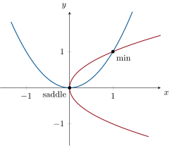
. Critical points: gives and , so : : points and .
Second derivatives: , , . At : : saddle. At : , : local minimum, . (Not global: .)
Example 25.16 (A four-point study, in full)
. Gradient:
Critical points: if , the second equation gives ; if , the first gives ; if , solve , : . Four points: , , , . Second derivatives: , , .
- : , , : , : local maximum, .
- : , : : saddle; likewise () and : three saddles.
The maximum is only local: . Symmetry check: , and indeed the critical set and the classification are symmetric in . Interpretation: among rectangles-with-slack , , the product of the three “parts” of is largest when the parts are equal — a two-variable shadow of the AM–GM principle.
Remark 25.17 (Common pitfalls)
Partial derivatives may exist at a point of discontinuity: the radial trap of Example 25.3 has (both axis restrictions vanish identically), yet has no limit at the origin — partials probe two directions only, continuity needs all of them; only the hypothesis restores order (Theorem 25.5). Line limits never suffice: Exercise 25.3’s function has limit along every line and still no limit — always try parabolas (or polar bounds valid uniformly in ). Critical is necessary, not sufficient: saddles abound (three of four points in Example 25.16); and the theorem holds on open sets only — on a closed disc, extrema may sit on the boundary with nonzero gradient (Exercise 25.12). The silent case is genuinely silent: (minimum) and (neither) both have at the origin; only a direct sign study decides (Exercise 25.6, function ). The gradient is orthogonal to level curves, not along them: to follow a contour line, move perpendicular to ; to climb fastest, move along it — mixing the two reverses the geometry of every contour map.
Remark 25.18 (Where two variables lead)
This chapter is a doorway. The gradient and the chain rule extend verbatim to variables in the Year 2 volume, where the of Theorem 25.5 becomes the differential and the Monge test is proved in full via the order-two Taylor formula and quadratic forms. The special case that can be settled this year — quadratic functions, for which the second-order expansion is exact — is the subject of the weekend problem, and it happens to be the case that runs the world’s data fitting: least squares regression. Constrained extrema (Exercise 25.5 was a preview) become Lagrange multipliers in Year 2; harmonic functions (Exercise 25.7) return in the complex analysis of the Year 3 volume.
Remark 25.19 (Perspectives inside Book 3: the year, closed)
This chapter is where the volume’s two halves shake hands. The analysis half supplied its tools one derivative at a time: the mean value theorem drives Theorem 25.5, Taylor expansions drive the extremum tests, and the ’s of Chapter 12 came back with balls instead of intervals. The algebra half supplied the geometry: the gradient is read through the inner product of Chapter 23 (Cauchy–Schwarz makes it the steepest direction), the Monge data is a symmetric matrix of Chapter 21 with the determinant test of Chapter 22, and the weekend problem runs orthogonal projection on data vectors. Even the curves of Chapter 24 return as level sets. A reader who can reconstruct why each of these five hand-offs works has, in effect, revised the entire year — which is the real purpose of this final chapter.
25.4 Exercises
Exercise 25.1 ★
Compute the partial derivatives: ; (on ); (on ).
Solution
Solution of Exercise 25.1.
, .
, .
, .
Exercise 25.2 ★
Study the continuity at (with value there) of:
(Polar coordinates , help: bound by a function of alone when possible.)
Solution
Solution of Exercise 25.2.
In polar coordinates ():
: continuous.
: independent of , taking different values along different rays (cf. Example 25.3): no limit, not continuous.
: continuous.
Exercise 25.3 ★★
Let (). Prove that has limit at the origin along every straight line, but that : is not continuous at .
Solution
Solution of Exercise 25.3.
Along : (for ; along and the -axis, ). So every straight-line limit is . But on the parabola :
the sequence has . Not continuous: lines do not suffice to test two-variable limits.
Exercise 25.4 ★
Verify Schwarz’s theorem by hand on .
Solution
Solution of Exercise 25.4.
; then
; then
equal, as Schwarz promises.
Exercise 25.5 ★★
Let be on and . Express via the chain rule. Deduce that restricted to the unit circle attains extrema at points where is parallel to the radius vector.
Solution
Solution of Exercise 25.5.
By Theorem 25.7 with :
At an extremum of , : is orthogonal to the tangent vector of the circle, hence parallel to the radius vector (the plane orthogonal complement of a unit vector is the line it spans, taken perpendicular). This is the simplest instance of a Lagrange multiplier.
Exercise 25.6 ★★
Find and classify the critical points of:
(For , the determinant test is silent at the origin: examine and .)
Solution
Solution of Exercise 25.6.
: : and : , . Second order: , , : , : local (indeed global — quadratic) minimum at , value .
: : point ; , , : : saddle.
: . Adding: , so ; substituting: : . Critical points: , , . At : , , : , : local minima (value ). At : , : : silent. Examine: and for small : both signs in every neighborhood — no extremum at the origin.
Exercise 25.7 ★★
A function is harmonic when . Check that , , and (off the origin) are harmonic.
Solution
Solution of Exercise 25.7.
: second partials and : sum . : both pure second partials vanish. : , : sum . : from Exercise 25.1,
and the -version is its opposite: sum .
Exercise 25.8 ★★★
Find the point of the plane closest to the origin, two ways: by orthogonal projection (Chapter 23), and by minimizing the two-variable function obtained by eliminating .
Solution
Solution of Exercise 25.8.
Projection: the plane has normal and passes through . The closest point to the origin is projected: , at distance . (Formula: distance from origin to plane is with .)
Minimization: . Writing for the last factor:
Substituting into the definition of : , so , giving , , and . Same point as by projection, at distance ; it is a minimum since at infinity (a positive-definite quadratic plus linear terms).
Exercise 25.9 ★★★
(Laplacian in polar coordinates, first contact) Let be on and radial: with of class on . Prove that
and find all radial harmonic functions on the punctured plane.
Solution
Solution of Exercise 25.9.
With : , so
(quotient and chain rules). Adding the symmetric -expression: the terms collect , the terms collect :
Radial harmonic: solve : the first-order equation for gives (Theorem 5.2), then . The radial harmonic functions are — the logarithmic potential of Exercise 25.7 and the constants, nothing else.
Exercise 25.10 ★★
Give the equation of the tangent plane to the graph at the point . Then find all points of the graph of where the tangent plane is horizontal, and relate the answer to Example 25.15.
Solution
Solution of Exercise 25.10.
For at : partials and , tangent plane . Horizontal tangent plane means both partials vanish, i.e. : by Example 25.15, exactly the critical points and , with horizontal planes and . “Horizontal tangent plane” and “critical point” are the same notion, seen on the graph and in the formula.
Exercise 25.11 ★★
Let be on .
- If everywhere, prove that depends only on .
- Find all solutions of the equation on . (Set and compute by the chain rule.)
Solution
Solution of Exercise 25.11.
- For fixed , the one-variable function has zero derivative on , hence is constant (Theorem 14.9): for all : depends only on .
Let . By the chain rule (Theorem 25.7, applied in the variable with frozen):
By (1), depends only on : with of class , and reversing the change of variables (, ),
Conversely every such satisfies : the solutions are exactly the functions of .
Exercise 25.12 ★★★
Find the global maximum and minimum of on the closed disc . (Admit the two-variable extreme value theorem: a continuous function on the closed disc attains its bounds — proved in the Year 2 volume. Treat the open disc by critical points and the boundary circle by the parametrization of Exercise 25.5.)
Solution
Solution of Exercise 25.12.
On the open disc, an extremum would be critical: only at , where ; it is a saddle (), so no extremum there. By the admitted extreme value theorem the bounds are attained, necessarily on the boundary circle. There, with Exercise 25.5,
with maximum at (points ) and minimum at (points ). Global maximum , global minimum .
25.5 Problem: least squares and the regression line
Problem 25.1
Given data points, which straight line passes “closest” to all of them? Legendre and Gauss answered: the line minimizing the sum of the squared vertical errors — because that minimization is exactly solvable by linear algebra. This problem first proves the Monge test of Method 25.14 honestly for quadratic functions (the one case where the second-order expansion is exact), then builds the normal equations, the regression line, and the correlation coefficient on top of the Euclidean geometry of Chapter 23.
Part I — Quadratic functions: the Monge test, proved. Fix reals and let .
Suppose . Establish the completed-square form
and deduce: if , has the strict sign of off the origin; if , takes both signs.
- Settle the remaining cases: , (symmetric); and (). Conclude: takes both signs iff , and vanishes only at the origin iff .
Let now be a quadratic function with a critical point . Prove the exact expansion
and deduce the Monge classification for quadratic functions: strict global minimum if , ; strict global maximum if , ; saddle if .
Suppose and (so also ). Prove the explicit coercivity bound
(Show that the quadratic form , with coefficients , , , still has nonnegative discriminant-test data.)
- Deduce that a quadratic function with positive definite quadratic part tends to as , and therefore has a unique global minimizer: its critical point. Contrast with Example 25.15, where a local minimum of a nonquadratic function was not global.
Part II — The normal equations. Let (canonical inner product), and
- Expand and show it is a quadratic function of with quadratic-part coefficients , , .
- Show that if and only if is free (the equality case of Cauchy–Schwarz, Theorem 23.4); assume this from now on.
Show that the critical equations are the normal equations
— the Gram matrix of Exercise 23.11 on the left — and that they say exactly: . Conclude with Part I and Theorem 23.10: the unique minimizer gives the orthogonal projection of onto .
- Show that the minimal value is , and draw the Pythagorean picture.
Part III — The regression line. Data points , not all equal. Minimize
Write , , , , .
Recognize Part II with , , , and write the normal equations
Solve them:
and observe that the regression line passes through the mean point .
- Check exactly when the are not all equal, and match this with question 7.
Prove that the minimal error is
Deduce , with if and only if the data are perfectly aligned.
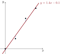
- Worked example: for the data , , , , compute , the regression line, the four residuals and .
- Prove that the residuals of the optimal line satisfy and , and interpret both via orthogonality.
Part IV — Variations and applications.
- (Best constant) Show that the constant minimizing is the mean , and that the minimal value is : the variance measures the failure of the data to be constant.
- (Line through the origin) Show that the slope minimizing is , and give a condition on the data for to coincide with the slope of question 11.
- (Distance to a line, again) For a point and the line through directed by the unit vector , minimize and deduce ; recover the formula for the line in the plane.
- (Analysis of variance) Prove the decomposition : the variance of the splits into the part explained by the line plus the residual variance.
(Parabolic fit) To fit , show that the normal equations are the system with the moment matrix
a Gram matrix which is invertible as soon as three of the are distinct (freeness of sampled at the data, Exercise 23.11; compare the moment matrices of the weekend problem of Chapter 22).
Part V — Robustness, and synthesis.
Classify the critical points of the three quadratic functions
by Part I, treating the degenerate third case by hand (where is the minimum attained?).
- (Outlier experiment) Append the point to the data of question 14 and recompute the slope . What happened, and why is the squared error so sensitive to one distant point?
- (Weighted least squares) Given weights , minimize : show the solution is given by the same formulas as question 11 with weighted means, variance and covariance (define them).
- Show that for the optimal line, forces all points to lie exactly on it, and connect with the equality case of question 13; test on the aligned data .
- Synthesis, in four sentences: why quadratic functions are the one class where this chapter’s second-order test needs no admitted theorem; how the normal equations identify the analytic minimization with the orthogonal projection of Chapter 23; what the correlation coefficient measures and which inequality bounds it; and which pieces of Chapters 18–23 (bases, Gram and moment matrices, projections) reappeared. Name the method and the equations studied in Parts II–III.
Solution
Solution of Problem 25.1.
1. Expanding the right-hand side:
If : both squares carry the factor sign of , and forces then : strict sign of off the origin. If : while has the opposite sign: both signs occur.
2. If , exchange the roles of and (the completed square in ), with the same conclusions; note as soon as , and indeed takes both signs then ( small against ). If : , both signs iff , i.e. iff . Summary: takes both signs ; vanishes only at the origin (definite) (which forces , since gives ).
3. With and , direct expansion gives
with no higher terms (the function is a polynomial of degree ). At a critical point the linear part vanishes: exactly, so the sign study of questions 1–2 classifies: strict global minimum (, ), strict global maximum (, ), saddle — both signs in every neighborhood — when . This proves Method 25.14 for quadratic functions.
4. The form has data , , . With (note since and ):
and (, true). If , the completed square of question 1 shows ; if , then (from forcing the displayed quantity with first factor ) and the form is . In both cases .
5. By questions 3–4, as : is coercive, and the inequality is strict for : the critical point is the unique global minimizer. For the cubic of Example 25.15, no such conclusion holds: , and the local minimum at is not global — exactness of the quadratic expansion is what failed.
6. Expanding the squared norm:
a quadratic function of whose quadratic part is with , , .
7. by Cauchy–Schwarz (Theorem 23.4), with equality exactly when are proportional (or one is zero), i.e. when the pair is linked. So free.
8. reads
the normal equations with the Gram matrix on the left; they say for , i.e. for . By Part I (questions 3, 5) the unique critical point is the unique global minimizer, and by Theorem 23.10 the characterization “, ” identifies as the orthogonal projection of onto .
9. , and gives : the minimum equals . Pythagoras: — the data vector splits into its explained part and its residual part , orthogonal to each other.
10. with the stated ; the normal equations of question 8 are, entrywise,
11. Dividing by : and . Substituting into the second: , so
and the first equation says precisely that lies on the line.
12. , zero iff every equals . And : question 7’s freeness condition is , i.e. the not all equal.
13. With , center the data (, ):
minimized at with value . Since and : , and iff , i.e. iff every residual vanishes: the points lie exactly on the line.
14. : , , so , so . Hence
Fitted values ; residuals ; (check: and ).
15. The two normal equations of question 10 are exactly and : the residual vector is orthogonal to and to — to the whole model space. In particular the optimal line always balances its errors: they sum to zero.
16. gives (and the second derivative makes it the global minimum, the function being a coercive quadratic in one variable). Minimal value : the variance is the irreducible quadratic error of a constant model.
17. gives . Writing both slopes over centered quantities: equals iff , i.e. iff (centered abscissas) or — the latter meaning : the full regression line already passes through the origin.
18. is minimal at , with value . In the plane, complete into an orthonormal basis with (unit normal of ): then , so , and with :
19. From and :
total variance variance along the fitted line residual variance. (Dividing by : , the share of variance “explained” by the line is .)
20. The model space is with , , ; minimizing leads, exactly as in question 8, to the Gram system, whose matrix has entries : the displayed moment matrix. It is invertible iff is free (Exercise 23.11); a relation for all makes every a root of one polynomial of degree , impossible with three distinct values unless . Compare the moment matrices of the weekend problem of Chapter 22, where their determinants were squared Vandermonde values.
21. First: , , : strict global minimum at the origin. Second: , : saddle. Third: , : degenerate — but vanishes on the whole line : a (non-strict) global minimum attained along a line, invisible to the determinant test.
22. New sums (): , , so , so . New slope:
one point turned a clearly increasing trend () into a slightly decreasing one. The squared error charges a residual , so a single distant point — large and large residual — dominates both and : least squares is efficient but not robust.
23. Set and define , likewise, , . The map is an inner product on ( gives definiteness), so Part II applies verbatim and the normal equations divide by into
whence and : the same formulas, with every average weighted.
24. forces every : all points exactly on the line; by question 13 this is the case . Test: for : , , , : , , and indeed for all three points; and .
25. (i) For quadratic functions the order-two expansion is an identity, so the sign study of the quadratic form — pure algebra, questions 1–2 — classifies critical points with no admitted Taylor theorem. (ii) The normal equations say “residual orthogonal to the model space”, so the analytic minimum is the orthogonal projection of the data vector: calculus and Euclidean geometry compute the same object. (iii) The correlation measures the share of the variance explained by the line, and Cauchy–Schwarz bounds it: , with equality only for aligned data. (iv) Bases and freeness (Chapter 18), Gram and moment matrices and their determinants (Chapters 22–23), and orthogonal projection (Chapter 23) all reappeared as the working parts of one algorithm. Parts II–III develop the method of least squares (Legendre, Gauss) through its normal equations.