University Mathematics — Year 1 · Bachelor Year 1

20Linear Maps

The maps worth studying between vector spaces are those compatible with the structure: linear maps. Their two fundamental subspaces — kernel and image — measure injectivity and surjectivity, and in finite dimension the rank–nullity theorem binds their sizes into one conservation law. Projections and symmetries, then linear forms and hyperplanes, close the chapter.

20.1 Definitions and first properties

Definition 20.1

Let $E, F$ be $K$ -vector spaces. A map $u \colon E \to F$ is linear when

\forall x, y \in E,\ \forall \lambda \in K, \qquad u(x + \lambda y) = u(x) + \lambda u(y).

Then $u(0) = 0$ and $u(\sum \lambda_i x_i) = \sum \lambda_i u(x_i)$ . The set $\mathcal{L}(E, F)$ of linear maps is itself a vector space; composition of linear maps is linear, and bilinear in the pair. An endomorphism is a linear $E \to E$ ; an isomorphism is a bijective linear map (its inverse is then automatically linear); $u^{-1}$ of an isomorphism, compositions of isomorphisms, are isomorphisms.

Proof that the inverse is linear. Let $u$ be linear bijective, $y, y' \in F$ and $\lambda \in K$ . Put $x = u^{-1}(y)$ and $x' = u^{-1}(y')$ . Then

u\bigl(x + \lambda x'\bigr) = u(x) + \lambda u(x') = y + \lambda y' ,

and applying $u^{-1}$ to both ends: $u^{-1}(y + \lambda y') = x + \lambda x' = u^{-1}(y) + \lambda\,u^{-1}(y')$ . Nothing about $u^{-1}$ was computed: linearity transports through the defining property of $u$ alone — a pattern worth remembering, as structure often rides along bijections for free. ∎

Proposition 20.2 (A linear map is known on a basis)

Let $(e_1, \dots, e_n)$ be a basis of $E$ and $(v_1, \dots, v_n)$ arbitrary vectors of $F$ . There is exactly one linear map $u \colon E \to F$ with $u(e_i) = v_i$ for all $i$ . Moreover:

u \text{ injective} \iff (v_i) \text{ free}; \qquad u \text{ surjective} \iff (v_i) \text{ generates } F .

Proof. Existence/uniqueness: every $x$ has unique coordinates $x = \sum \lambda_i e_i$ (Proposition 18.15); linearity forces $u(x) = \sum \lambda_i v_i$ , and this formula does define a linear map.

Injectivity: by Proposition 20.5 below, $u$ is injective iff its kernel is trivial. Now $u\bigl(\sum\lambda_i e_i\bigr) = 0$ means exactly $\sum\lambda_i v_i = 0$ . If $(v_i)$ is free, this forces every $\lambda_i = 0$ , i.e. the kernel reduces to $0$ : injective. If $(v_i)$ is linked, a nontrivial relation $\sum\lambda_i v_i = 0$ produces the nonzero vector $\sum\lambda_i e_i$ in the kernel ( $(e_i)$ is free): not injective. The two conditions match term for term.

Surjectivity: the image of $u$ is the set of all $\sum\lambda_i v_i$ , i.e. exactly $\operatorname{Vect}(v_1, \dots, v_n)$ , which equals $F$ iff the family generates. ∎

Definition 20.3 (Kernel and image)

For $u \in \mathcal{L}(E, F)$ :

\ker u = \{x \in E : u(x) = 0\} \subseteq E, \qquad \operatorname{im} u = u(E) \subseteq F ,

both subspaces (direct verification with the criterion).

Method 20.4 (Kernel and image, in practice)

Kernel: write $u(x) = 0$ as a system on the coordinates (or coefficients) of $x$ , solve, and parametrize — the kernel comes out with a basis attached (Method 19.10). Image: it is the span of the images of any generating family of $E$ — usually a basis, so $\operatorname{im} u = \operatorname{Vect}\bigl(u(e_1), \dots, u(e_n)\bigr)$ ; then eliminate redundant images to extract a basis. Shortcut: compute whichever of the two is easier and get the other’s dimension for free by rank–nullity (Theorem 20.7); when a plausible candidate subspace for the image is known, comparing dimensions upgrades the easy inclusion to equality (Theorem 19.14). Both shortcuts are used in Example 20.11 below.

Proposition 20.5

$u$ is injective $\iff$ $\ker u = \{0\}$ ; $u$ is surjective $\iff$ $\operatorname{im} u = F$ .

Proof. As for groups (Proposition 7.11): $u(x) = u(y) \iff u(x - y) = 0 \iff x - y \in \ker u$ . The second point is the definition. ∎

20.2 The rank–nullity theorem

Definition 20.6

The rank of $u \in \mathcal{L}(E, F)$ (with $E$ finite-dimensional) is $\operatorname{rk} u = \dim \operatorname{im} u$ — also the rank of the family $\bigl(u(e_1), \dots, u(e_n)\bigr)$ for any basis $(e_i)$ of $E$ .

Theorem 20.7 (Rank–nullity)

Let $E$ be finite-dimensional and $u \in \mathcal{L}(E, F)$ . Then

\dim E = \dim \ker u + \operatorname{rk} u .

More precisely, if $S$ is any supplementary subspace of $\ker u$ in $E$ , then $u$ restricts to an isomorphism from $S$ onto $\operatorname{im} u$ .

Proof. Let $S$ satisfy $E = \ker u \oplus S$ (Theorem 19.14), and let $v \colon S \to \operatorname{im} u$ be the restriction of $u$ .

$v$ is injective: $\ker v = S \cap \ker u = \{0\}$ .

$v$ is surjective: any $u(x)$ with $x = k + s$ ( $k \in \ker u$ , $s \in S$ ) equals $u(s) = v(s)$ .

So $v$ is an isomorphism; an isomorphism sends a basis to a basis (Proposition 20.2), so $\dim S = \dim\operatorname{im} u$ , and $\dim E = \dim\ker u + \dim S$ concludes. ∎

Example 20.8 (Building a map to specification)

Construct $u \in \mathcal{L}(\R^3)$ with $\ker u = \operatorname{Vect}(1,1,1)$ and $\operatorname{im} u = \{z = 0\}$ . Sanity first: rank–nullity demands $1 + 2 = 3$ — consistent, so a solution may exist. Choose a basis adapted to the kernel, say $\bigl((1,1,1),\ e_1,\ e_2\bigr)$ (Example 19.7), and prescribe images (Proposition 20.2):

u(1,1,1) = 0, \qquad u(e_1) = e_1, \qquad u(e_2) = e_2 .

Then $\ker u \supseteq \operatorname{Vect}(1,1,1)$ and $\operatorname{im} u = \operatorname{Vect}(e_1, e_2) = \{z = 0\}$ ; rank–nullity forces $\dim\ker u = 1$ , so the kernel is exactly the prescribed line. Explicitly, decomposing $(x, y, z) = z(1,1,1) + (x - z)e_1 + (y - z)e_2$ :

u(x, y, z) = (x - z,\ y - z,\ 0).

The recipe generalizes: a linear map with prescribed kernel $N$ and image $I$ exists exactly when $\dim N + \dim I = \dim E$ — necessity is rank–nullity, sufficiency is this construction.

Corollary 20.9

If $\dim E = \dim F$ (finite), then for $u \in \mathcal{L}(E, F)$ :

u \text{ injective} \iff u \text{ surjective} \iff u \text{ bijective}.

In particular this holds for endomorphisms in finite dimension. (It fails in infinite dimension: on $K[X]$ , the derivative is surjective but not injective, and $P \mapsto XP$ is injective but not surjective.)

Proof. Injective $\iff \dim\ker u = 0 \iff \operatorname{rk} u = \dim E = \dim F \iff \operatorname{im} u = F$ (a subspace of full dimension is everything, Theorem 19.14) $\iff$ surjective. ∎

Example 20.10 (Interpolation, structurally)

Fix distinct $x_0, \dots, x_n$ and let $u \colon \R_n[X] \to \R^{n+1}$ , $P \mapsto (P(x_0), \dots, P(x_n))$ : linear. Its kernel is $\{P : \deg P \leq n,\ n+1 \text{ roots}\} = \{0\}$ (Corollary 8.8). Equal dimensions $n + 1$ : $u$ is an isomorphism — existence and uniqueness of the Lagrange interpolant (Theorem 8.23) in one line.

The same one-line pattern handles data mixing values and derivatives: $v \colon \R_3[X] \to \R^4$ , $P \mapsto \bigl(P(0), P'(0), P(1), P'(1)\bigr)$ is linear, and its kernel consists of degree- $\leq 3$ polynomials with double roots at $0$ and $1$ , i.e. divisible by $X^2(X-1)^2$ of degree $4$ : only $P = 0$ . Equal dimensions again: every quadruple of data $(P(0), P'(0), P(1), P'(1))$ is realized by exactly one cubic — Hermite interpolation, granted by a kernel computation before any formula is written (the weekend problem of Chapter 22 meets its determinant).

Example 20.11 (Rank–nullity at work: the difference operator)

Let $\Delta \colon \R_n[X] \to \R_n[X]$ , $P \mapsto P(X+1) - P(X)$ : linear. Kernel: if $\Delta P = 0$ , then $P(0) = P(1) = P(2) = \dots$ , so $P - P(0)$ has infinitely many roots and vanishes (Corollary 8.8): $\ker\Delta$ is the line of constants. Rank–nullity: $\operatorname{rk}\Delta = (n + 1) - 1 = n$ . Since $\deg \Delta P < \deg P$ for nonconstant $P$ (the top terms cancel), $\operatorname{im}\Delta \subseteq \R_{n-1}[X]$ , which has dimension exactly $n$ : the inclusion is an equality. Conclusion, with no computation of preimages: every polynomial $Q$ of degree $\leq n - 1$ is a difference $Q = P(X+1) - P(X)$ — the discrete antiderivative exists. (Compare the weekend problem of Chapter 18, where $\Delta$ was inverted explicitly in the binomial basis.)

Example 20.12 (Rank bookkeeping along a composition)

On $\R_2[X]$ , compose the derivative $D(P) = P'$ (rank $2$ : image $\R_1[X]$ , kernel the constants) with itself. Then $D \circ D = D^2$ maps $P \mapsto P''$ , with image $\R_0[X]$ : rank $1$ . Compare with the general bounds: the crude one gives $\operatorname{rk} D^2 \leq \min(2, 2) = 2$ ; the exact formula of Exercise 20.12 accounts for the loss precisely,

\operatorname{rk} D^2 = \operatorname{rk} D - \dim\bigl(\ker D \cap \operatorname{im} D\bigr) = 2 - 1 = 1 ,

since the constants (kernel of the outer $D$ ) sit inside $\R_1[X]$ (image of the inner $D$ ) with dimension $1$ . Rank is lost exactly where the outer kernel ambushes the inner image — the sentence to remember when composition ranks misbehave.

Example 20.13 (Kernel and image of the Euler operator)

On $\R_n[X]$ , let $u(P) = X\,P'$ (linear: differentiation and multiplication by $X$ are). Kernel: $XP' = 0$ forces $P' = 0$ (a product of polynomials vanishes only if one factor does), so $\ker u$ is the line of constants. Image: on the monomial basis,

u(X^k) = k\,X^{k} \qquad (k = 0, 1, \dots, n),

so $\operatorname{im} u = \operatorname{Vect}(X, 2X^2, \dots, nX^n) = \operatorname{Vect}(X, X^2, \dots, X^n)$ : the polynomials with zero constant term. Check against rank–nullity: $\operatorname{rk} u = (n + 1) - 1 = n$ , which is indeed the dimension found. Two remarks worth keeping. First, here $\operatorname{im} u \oplus \ker u = \R_n[X]$ — but that is a happy accident of this operator, not a theorem: for the shift-like $v(P) = P'$ on $\R_1[X]$ , $\ker v = \operatorname{im} v = \R_0[X]$ and the sum is not direct. Second, the relation $u(X^k) = kX^k$ says each monomial is merely rescaled by $u$ — a basis adapted to the map, the germ of the eigenvalue idea developed in the Year 2 volume.

20.3 Projections and symmetries

Definition 20.14

Let $E = F \oplus G$ . The projection onto $F$ along $G$ maps $x = f + g$ (unique decomposition) to $p(x) = f$ ; the associated symmetry is $s(x) = f - g$ . Both are linear, and $s = 2p - \mathrm{id}$ .

Theorem 20.15 (Algebraic characterization)

An endomorphism $p$ is a projection (onto some $F$ along some $G$ ) if and only if $p \circ p = p$ ; then $F = \operatorname{im} p = \ker(p - \mathrm{id})$ and $G = \ker p$ .
An endomorphism $s$ is a symmetry if and only if $s \circ s = \mathrm{id}$ ; then $E = \ker(s - \mathrm{id}) \oplus \ker(s + \mathrm{id})$ .

Proof. (1) A projection satisfies $p(f + g) = f$ and $p(f) = f$ : $p^2 = p$ . Conversely, let $p^2 = p$ ; set $F = \operatorname{im} p$ , $G = \ker p$ . Every $x$ writes $x = p(x) + (x - p(x))$ with $p(x) \in F$ and $p\bigl(x - p(x)\bigr) = p(x) - p^2(x) = 0$ : $E = F + G$ . If $y \in F \cap G$ : $y = p(z)$ and $p(y) = 0$ , so $y = p(z) = p^2(z) = p(y) = 0$ : direct sum, and $p$ is the projection onto $F$ along $G$ . Finally on $F$ : $y = p(z)$ gives $p(y) = y$ , so $F \subseteq \ker(p - \mathrm{id})$ , and conversely $p(y) = y$ puts $y$ in the image.

(2) The correspondence $s = 2p - \mathrm{id}$ , $p = \frac{s + \mathrm{id}}2$ is a bijection between endomorphisms, and under it

s^2 = 4p^2 - 4p + \mathrm{id} = \mathrm{id} \iff 4p^2 = 4p \iff p^2 = p :

symmetries correspond exactly to projections. Translating the subspaces: $s(x) = x \iff p(x) = x$ , so $\ker(s - \mathrm{id}) = \operatorname{im} p = F$ ; and $s(x) = -x \iff 2p(x) = 0 \iff x \in \ker p = G$ , so $\ker(s + \mathrm{id}) = G$ . The direct sum $E = F \oplus G$ of point (1) becomes the announced decomposition into the fixed vectors and the reversed vectors of $s$ . ∎

Example 20.16 (A projection and its symmetry, explicitly)

In $\R^2$ , project onto $F = \operatorname{Vect}(1,1)$ along $G = \operatorname{Vect}(0,1)$ . Decompose $(x, y) = a(1,1) + b(0,1)$ : the first coordinate gives $a = x$ , the second $b = y - x$ . Hence

p(x, y) = (x, x), \qquad s(x, y) = 2p(x,y) - (x,y) = (x,\ 2x - y).

Check the algebra: $p(p(x,y)) = p(x,x) = (x,x)$ , and $s(s(x,y)) = s(x, 2x - y) = (x, 2x - (2x - y)) = (x, y)$ . Geometrically, $s$ is the “oblique reflection” across the line $y = x$ in the vertical direction: it fixes $F$ pointwise and reverses $G$ . Had we projected onto the same $F$ along $G' = \operatorname{Vect}(1,-1)$ instead, the formula would change to $p'(x,y) = \bigl(\frac{x+y}2, \frac{x+y}2\bigr)$ : a projection is determined by its image and its kernel, never by the image alone.

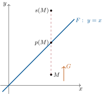
The projection onto F = Vect(1,1) along G = Vect(0,1) and its symmetry, on the point M = (2,\ 0.5): sliding vertically, M hits F at p(M) = (2,2) and lands at s(M) = 2p(M) - M = (2,\ 3.5), as far above F (measured along G) as M was below. — The projection onto $F = \operatorname{Vect}(1,1)$ along $G = \operatorname{Vect}(0,1)$ and its symmetry, on the point $M = (2,\ 0.5)$ : sliding vertically, $M$ hits $F$ at $p(M) = (2,2)$ and lands at $s(M) = 2p(M) - M = (2,\ 3.5)$ , as far above $F$ (measured along $G$ ) as $M$ was below.

20.4 Linear forms and hyperplanes

Definition 20.17

A linear form on $E$ is a linear map $\varphi \colon E \to K$ . A hyperplane of $E$ ( $\dim E = n$ ) is a subspace of dimension $n - 1$ .

Example 20.18 (An evaluation form and its hyperplane)

On $\R_2[X]$ , the evaluation $\varphi(P) = P(2)$ is a linear form, nonzero ( $\varphi(1) = 1$ ). Its kernel is the hyperplane of polynomials vanishing at $2$ , i.e. (factor theorem, Theorem 8.7) the multiples of $X - 2$ within $\R_2[X]$ :

\ker\varphi = \operatorname{Vect}\bigl(X - 2,\ X(X - 2)\bigr), \qquad \dim = 2 .

In coordinates on $(1, X, X^2)$ , $\varphi(a + bX + cX^2) = a + 2b + 4c$ : every linear form on a finite-dimensional space is, once a basis is fixed, a fixed linear expression in the coordinates — forms are “row vectors”, as Chapter 21 will make literal, and the coefficient row here, $(1, 2, 4)$ , is a Vandermonde row: evaluation forms are how the interpolation theory of Chapter 22’s weekend problem enters linear algebra.

Theorem 20.19

The hyperplanes of $E$ are exactly the kernels of nonzero linear forms. Two nonzero forms have the same kernel if and only if they are proportional.

Proof. If $\varphi \neq 0$ : $\operatorname{rk}\varphi = 1$ (image a nonzero subspace of $K$ ), so $\dim\ker\varphi = n - 1$ : a hyperplane. Conversely, let $H$ be a hyperplane, $(e_1, \dots, e_{n-1})$ a basis of $H$ completed by $e_n$ : the form “last coordinate” has kernel $H$ .

Proportional forms share their kernel. Conversely, suppose $\ker\varphi = \ker\psi = H$ and pick $a \notin H$ : every $x$ writes $x = h + \lambda a$ (as $E = H \oplus Ka$ ), and

\varphi(x) = \lambda \varphi(a), \qquad \psi(x) = \lambda\psi(a):

so $\varphi = \frac{\varphi(a)}{\psi(a)}\,\psi$ . ∎

Example 20.20

In $K^n$ , a hyperplane is a solution set $\{a_1 x_1 + \dots + a_n x_n = 0\}$ with not all $a_i$ zero — the familiar equation of a plane through the origin in $\R^3$ . In function spaces, evaluation forms $P \mapsto P(1)$ or $f \mapsto \int_0^1 f$ define hyperplanes of $\R_n[X]$ , of $C(\intcc{0}{1})$ (cf. Exercise 19.6).

Example 20.21 (One hyperplane, worked three ways)

Take $\varphi(x, y, z) = x - 2y + 3z$ on $\R^3$ and $H = \ker\varphi$ . Basis: solve $x = 2y - 3z$ :

(2y - 3z,\ y,\ z) = y\,(2, 1, 0) + z\,(-3, 0, 1),

two free vectors: $\dim H = 2$ , a hyperplane, as Theorem 20.19 predicts from $\varphi \neq 0$ . Supplementary line: any vector outside $H$ spans one, e.g. $a = (1, 0, 0)$ ( $\varphi(a) = 1 \neq 0$ ); the decomposition of an arbitrary $v$ is explicit:

v = \underbrace{\bigl(v - \varphi(v)\,a\bigr)}_{\in\,H} + \underbrace{\varphi(v)\,a}_{\in\,\operatorname{Vect}(a)},

since $\varphi\bigl(v - \varphi(v)a\bigr) = \varphi(v) - \varphi(v)\varphi(a) = 0$ . Proportionality: if $\psi(x,y,z) = -2x + 4y - 6z$ , then $\psi = -2\varphi$ and both have kernel $H$ ; conversely, any form vanishing on $H$ is a multiple of $\varphi$ (Exercise 20.8) — the equation of a hyperplane is unique up to scale, a fact used constantly for planes in geometry.

Remark 20.22 (Common pitfalls)

Kernel and image live in different spaces: $\ker u \subseteq E$ , $\operatorname{im} u \subseteq F$ ; the sum $\ker u + \operatorname{im} u$ only makes sense for endomorphisms, and even then it need not be direct ( $u(x, y) = (y, 0)$ has $\ker u = \operatorname{im} u$ ; Exercise 20.7 characterizes when directness holds). $u^2 = 0$ does not mean $u = 0$ : the same $u(x,y) = (y, 0)$ squares to zero without vanishing — what $u^2 = 0$ really says is $\operatorname{im} u \subseteq \ker u$ (Exercise 20.5). Injective $\iff$ surjective needs equal finite dimensions: on $K[X]$ , the derivative is surjective and not injective, $P \mapsto XP$ injective and not surjective (Corollary 20.9); and between spaces of different dimensions, one implication is simply impossible ( $\operatorname{rk} u \leq \min(\dim E, \dim F)$ ). Prescribing images works on a basis, not on any family: demanding $u(1, 0) = a$ , $u(0, 1) = b$ , $u(1, 1) = c$ overdetermines $u$ unless $c = a + b$ ; a linear map is free on a basis, enslaved everywhere else. Rank is not preserved by composition: it can only drop, $\operatorname{rk}(vu) \leq \min(\operatorname{rk} u, \operatorname{rk} v)$ (Exercise 20.4), with exact loss measured in Exercise 20.12.

Remark 20.23 (Where these maps go)

Linear maps are about to become matrices: once bases are fixed, Chapter 21 encodes every $u \in \mathcal{L}(E, F)$ by a rectangular array, and composition becomes the matrix product — rank–nullity then drives the theory of linear systems in Chapter 22. Projections return in Chapter 23 in their most useful special case, the orthogonal projection, where the kernel is chosen perpendicular to the image. The weekend problem below pushes the projector algebra as far as first-year tools reach, up to Fitting’s lemma; the Year 2 volume goes further with the trace and with eigenvalue theory, for which projectors onto stable subspaces are the basic building blocks.

Remark 20.24 (Perspectives inside Book 3: rank–nullity three more times)

The conservation law $\dim E = \dim\ker u + \operatorname{rk} u$ will be re-read three times before the volume ends. In Chapter 22 it becomes the shape of solution sets: a compatible system with $p$ unknowns and rank $r$ has a solution set of dimension $p - r$ — kernel dimension in disguise. In Chapter 23 it splits orthogonally, $\dim F + \dim F^\perp = \dim E$ , and powers every distance computation. In the weekend problem of Chapter 25, it is the accountant of least squares: $n$ observations, $2$ fitted parameters, $n - 2$ residual dimensions, and the Pythagorean identity $\norm b^2 = \norm p^2 + \norm{b - p}^2$ is rank–nullity’s Euclidean shadow. One theorem, four costumes.

20.5 Exercises

Exercise 20.1 ★

Which maps are linear?

$\R^2 \to \R^2$ , $(x, y) \mapsto (x + y, x - 2y)$ ;
$\R^2 \to \R$ , $(x, y) \mapsto xy$ ;
$\R[X] \to \R[X]$ , $P \mapsto P' + XP$ ;
$\mathcal{F}(\R,\R) \to \R$ , $f \mapsto f(3)$ .

Solution

Solution of Exercise 20.1.

(1) Linear: coordinates are linear expressions. (2) Not linear: $u(2(1,1)) = 4 \neq 2 = 2u(1,1)$ . (3) Linear: differentiation and multiplication by $X$ are, and sums of linear maps are. (4) Linear: evaluation respects pointwise operations.

Exercise 20.2 ★

Let $u \colon \R^3 \to \R^3$ , $(x,y,z) \mapsto (x + y - z,\; 2x + y + z,\; 3x + 2y)$ . Determine $\ker u$ (basis, dimension), $\operatorname{rk} u$ , and a basis of $\operatorname{im} u$ . Is $u$ injective? surjective?

Solution

Solution of Exercise 20.2.

Kernel: solve $x + y - z = 0$ , $2x + y + z = 0$ , $3x + 2y = 0$ . From the third, $y = -\frac{3x}{2}$ ; the first gives $z = x + y = -\frac x2$ ; check in the second: $2x - \frac{3x}{2} - \frac x2 = 0$ : satisfied. So $\ker u = \operatorname{Vect}\bigl((2, -3, -1)\bigr)$ (taking $x = 2$ ), dimension $1$ .

Rank–nullity: $\operatorname{rk} u = 3 - 1 = 2$ . Image: spanned by the images of the canonical basis, $u(e_1) = (1,2,3)$ , $u(e_2) = (1,1,2)$ , $u(e_3) = (-1,1,0)$ ; the first two are free, and the rank is $2$ : basis $\bigl((1,2,3), (1,1,2)\bigr)$ .

Not injective ( $\ker \neq \{0\}$ ), not surjective (rank $2 < 3$ ): consistent with Corollary 20.9.

Exercise 20.3 ★

Let $u \colon \R_n[X] \to \R_n[X]$ , $P \mapsto P - P'$ . Prove that $u$ is an isomorphism: once via $\ker u$ , once by exhibiting the inverse (consider $P + P' + P'' + \dots$ ).

Solution

Solution of Exercise 20.3.

Kernel: $P = P'$ forces $\deg P = \deg P'$ unless $P = 0$ ; but $\deg P' < \deg P$ for $P \neq 0$ : so $\ker u = \{0\}$ , and $u$ , an injective endomorphism of the finite-dimensional $\R_n[X]$ , is an isomorphism (Corollary 20.9).

Inverse: let $v(P) = P + P' + P'' + \dots + P^{(n)}$ (a finite sum on $\R_n[X]$ ). Then

v\bigl(u(P)\bigr) = \sum_{k=0}^{n} (P - P')^{(k)} = \sum_{k=0}^{n} P^{(k)} - \sum_{k=0}^{n} P^{(k+1)} = P - P^{(n+1)} = P ,

telescoping, since $P^{(n+1)} = 0$ . So $v = u^{-1}$ .

Exercise 20.4 ★

Let $u \in \mathcal{L}(E, F)$ and $v \in \mathcal{L}(F, G)$ , spaces finite-dimensional. Prove:

\operatorname{rk}(v \circ u) \leq \min\bigl(\operatorname{rk} u,\ \operatorname{rk} v\bigr).

Solution

Solution of Exercise 20.4.

$\operatorname{im}(v \circ u) = v(\operatorname{im} u) \subseteq \operatorname{im} v$ : rank $\leq \operatorname{rk} v$ . And $v$ restricted to $\operatorname{im} u$ has image $\operatorname{im}(vu)$ with rank–nullity inside $\operatorname{im} u$ : $\operatorname{rk}(vu) \leq \dim\operatorname{im} u = \operatorname{rk} u$ .

Exercise 20.5 ★★

Let $u$ be an endomorphism of $E$ (finite-dimensional) with $u^2 = 0$ . Prove that $\operatorname{im} u \subseteq \ker u$ , hence $\operatorname{rk} u \leq \frac{\dim E}{2}$ . For $E = \R^2$ , give an example with equality.

Solution

Solution of Exercise 20.5.

$u^2 = 0$ means $u(u(x)) = 0$ for all $x$ : every $u(x)$ lies in $\ker u$ , i.e. $\operatorname{im} u \subseteq \ker u$ . Then rank–nullity:

\dim E = \dim\ker u + \operatorname{rk} u \geq 2\operatorname{rk} u .

Equality example in $\R^2$ : $u(x, y) = (y, 0)$ : $u^2 = 0$ , $\operatorname{rk} u = 1 = \frac{\dim E}{2}$ .

Exercise 20.6 ★★

Let $p, q$ be projections of $E$ with $p \circ q = q \circ p$ . Prove that $p \circ q$ is a projection, with

\operatorname{im}(pq) = \operatorname{im} p \cap \operatorname{im} q , \qquad \ker (pq) = \ker p + \ker q .

Solution

Solution of Exercise 20.6.

$(pq)^2 = pqpq = ppqq = pq$ (commutation): a projection (Theorem 20.15).

Image: $\operatorname{im}(pq) \subseteq \operatorname{im} p$ , and $= \operatorname{im}(qp) \subseteq \operatorname{im} q$ : contained in the intersection. Conversely, if $x \in \operatorname{im} p \cap \operatorname{im} q$ , then $p(x) = x$ and $q(x) = x$ (fixed points characterize the image of a projection), so $pq(x) = x$ : $x \in \operatorname{im}(pq)$ .

Kernel: $\ker p \subseteq \ker(qp) = \ker(pq)$ and likewise $\ker q \subseteq \ker(pq)$ : the sum is contained. Conversely, let $pq(x) = 0$ , and write

x = \underbrace{q(x)}_{\in\, \ker p} + \underbrace{(x - q(x))}_{\in\, \ker q} :

the first term satisfies $p(q(x)) = 0$ , so it lies in $\ker p$ ; the second is in $\ker q$ since $q(x - q(x)) = q(x) - q^2(x) = 0$ . Hence $x \in \ker p + \ker q$ .

Exercise 20.7 ★★

Let $u \in \mathcal{L}(E)$ , $E$ finite-dimensional. Prove the equivalence of:

$E = \ker u \oplus \operatorname{im} u$ ;
$\ker u = \ker u^2$ ;
$\operatorname{im} u = \operatorname{im} u^2$ .

Solution

Solution of Exercise 20.7.

Note first the general inclusions $\ker u \subseteq \ker u^2$ and $\operatorname{im} u^2 \subseteq \operatorname{im} u$ , and by rank–nullity, (2) $\iff$ (3) (equal kernels $\iff$ equal ranks $\iff$ equal images, given the inclusions).

(1 $\Rightarrow$ 2): let $u^2(x) = 0$ ; then $u(x) \in \ker u \cap \operatorname{im} u = \{0\}$ , so $x \in \ker u$ .

(2 $\Rightarrow$ 1): by Grassmann and rank–nullity, $\dim(\ker u + \operatorname{im} u) = \dim\ker u + \operatorname{rk} u - \dim(\ker u \cap \operatorname{im} u) = \dim E - \dim(\ker u \cap \operatorname{im} u)$ : the sum is $E$ iff the intersection is $\{0\}$ . Let $y \in \ker u \cap \operatorname{im} u$ : $y = u(x)$ and $u(y) = 0$ , so $u^2(x) = 0$ , so (by (2)) $u(x) = 0$ : $y = 0$ . Hence $E = \ker u \oplus \operatorname{im} u$ .

Exercise 20.8 ★★

Let $\varphi, \psi$ be linear forms on $E$ with $\ker\varphi \subseteq \ker\psi$ . Prove $\psi = \lambda\varphi$ for some $\lambda \in K$ (including the degenerate cases).

Solution

Solution of Exercise 20.8.

If $\varphi = 0$ : then $\ker\varphi = E \subseteq \ker\psi$ forces $\psi = 0 = 0\cdot\varphi$ . If $\varphi \neq 0$ : $\ker\varphi$ is a hyperplane; pick $a \notin \ker\varphi$ . Set $\lambda = \frac{\psi(a)}{\varphi(a)}$ . The form $\psi - \lambda\varphi$ vanishes on $\ker\varphi$ (both do, by the inclusion) and at $a$ : it vanishes on $\ker\varphi \oplus Ka = E$ . So $\psi = \lambda\varphi$ .

Exercise 20.9 ★★★

Let $u \in \mathcal{L}(E)$ with $\dim E = n$ , and suppose $u^n = 0$ but $u^{n-1} \neq 0$ (a maximally nilpotent endomorphism). Pick $x$ with $u^{n-1}(x) \neq 0$ ; prove that $\bigl(x, u(x), \dots, u^{n-1}(x)\bigr)$ is a basis of $E$ . (Apply powers of $u$ to a null combination, starting with $u^{n-1}$ .)

Solution

Solution of Exercise 20.9.

Suppose $\lambda_0 x + \lambda_1 u(x) + \dots + \lambda_{n-1} u^{n-1}(x) = 0$ . Apply $u^{n-1}$ : all terms with a factor $u^{\geq n}$ die, leaving $\lambda_0 u^{n-1}(x) = 0$ , so $\lambda_0 = 0$ . Apply $u^{n-2}$ to the remaining relation: $\lambda_1 u^{n-1}(x) = 0$ , so $\lambda_1 = 0$ ; and so on. The family is free; being of size $n = \dim E$ , it is a basis (Proposition 19.8). (In this basis, $u$ acts as a shift — the model of maximal nilpotence.)

Exercise 20.10 ★★★

Let $f \in \mathcal{L}(\R^n)$ with $f \circ f = -\mathrm{id}$ .

Prove that $f$ is an isomorphism and that no $x \neq 0$ satisfies $f(x) = \lambda x$ with $\lambda \in \R$ .
Prove that $n$ is even. Hint: pick $x_1 \neq 0$ ; show $\operatorname{Vect}(x_1, f(x_1))$ is a plane stable under $f$ ; choose $x_2$ outside it and iterate, proving that $\bigl(x_1, f(x_1), x_2, f(x_2), \dots\bigr)$ stays free.

Solution

Solution of Exercise 20.10.

$f \circ f = -\mathrm{id}$ is bijective, so $f$ is (Proposition 1.26 adapted: $f$ has the two-sided inverse $-f$ ). If $f(x) = \lambda x$ with $x \neq 0$ : applying $f$ , $-x = \lambda^2 x$ , so $\lambda^2 = -1$ : impossible in $\R$ .
Build the family greedily. Take $x_1 \neq 0$ : $(x_1, f(x_1))$ is free by (1). If $\operatorname{Vect}$ of the current family $\bigl(x_1, f(x_1), \dots, x_k, f(x_k)\bigr)$ , call it $V_k$ — a subspace stable under $f$ (each generator maps to another generator or its negative: $f(f(x_i)) = -x_i$ ) — is not all of $E$ , choose $x_{k+1} \notin V_k$ . Claim: the enlarged family is free. Suppose $\alpha x_{k+1} + \beta f(x_{k+1}) + v = 0$ with $v \in V_k$ and $(\alpha, \beta) \neq (0,0)$ . Apply $f$ : $\alpha f(x_{k+1}) - \beta x_{k+1} + f(v) = 0$ with $f(v) \in V_k$ . Eliminate $f(x_{k+1})$ between the two relations (multiply the first by $\alpha$ , the second by $-\beta$ , and add):

$(\alpha^2 + \beta^2)\, x_{k+1} \in V_k ,$

and $\alpha^2 + \beta^2 \neq 0$ forces $x_{k+1} \in V_k$ : contradiction. So the construction continues, adding vectors two at a time, until $V_k = E$ : the final family is a basis of even size, and $n$ is even.

Exercise 20.11 ★★

Let $u, v \in \mathcal{L}(E, F)$ , spaces finite-dimensional. Prove the two-sided bound

\abs{\operatorname{rk} u - \operatorname{rk} v} \;\leq\; \operatorname{rk}(u + v) \;\leq\; \operatorname{rk} u + \operatorname{rk} v .

(For the upper bound, compare $\operatorname{im}(u+v)$ with $\operatorname{im} u + \operatorname{im} v$ ; for the lower one, apply the upper bound cleverly.)

Solution

Solution of Exercise 20.11.

Upper bound: for every $x$ , $(u + v)(x) = u(x) + v(x) \in \operatorname{im} u + \operatorname{im} v$ , so

\operatorname{rk}(u + v) \leq \dim(\operatorname{im} u + \operatorname{im} v) \leq \operatorname{rk} u + \operatorname{rk} v

(Grassmann, Theorem 19.18). Lower bound: apply the upper bound to the pair $(u + v, -v)$ , whose sum is $u$ :

\operatorname{rk} u \leq \operatorname{rk}(u + v) + \operatorname{rk}(-v) = \operatorname{rk}(u + v) + \operatorname{rk} v,

so $\operatorname{rk} u - \operatorname{rk} v \leq \operatorname{rk}(u+v)$ ; exchanging $u$ and $v$ gives the absolute value.

Exercise 20.12 ★★★

(Frobenius’ inequality) Let $u \in \mathcal{L}(E, F)$ , $w \in \mathcal{L}(F, G)$ and $v \in \mathcal{L}(G, H)$ , all spaces finite-dimensional. Prove the exact formula

\operatorname{rk}(v \circ w) = \operatorname{rk} w - \dim\bigl(\ker v \cap \operatorname{im} w\bigr),

and deduce Frobenius’ inequality

\operatorname{rk}(v \circ w) + \operatorname{rk}(w \circ u) \;\leq\; \operatorname{rk} w + \operatorname{rk}(v \circ w \circ u) .

Check that the case $w = \mathrm{id}_F$ is Sylvester’s inequality, proved in matrix form in Exercise 21.10.

Solution

Solution of Exercise 20.12.

Exact formula. Let $v'$ be the restriction of $v$ to the subspace $\operatorname{im} w$ . Its image is $v(w(F)) = \operatorname{im}(v \circ w)$ , and its kernel is $\ker v \cap \operatorname{im} w$ . Rank–nullity for $v'$ on the space $\operatorname{im} w$ :

\operatorname{rk} w = \dim\operatorname{im} w = \operatorname{rk}(v \circ w) + \dim(\ker v \cap \operatorname{im} w) .

Frobenius. Apply the exact formula twice, to $w$ and to $w \circ u$ :

\operatorname{rk} w - \operatorname{rk}(vw) = \dim\bigl(\ker v \cap \operatorname{im} w\bigr), \qquad \operatorname{rk}(wu) - \operatorname{rk}(vwu) = \dim\bigl(\ker v \cap \operatorname{im}(wu)\bigr) .

Since $\operatorname{im}(w \circ u) \subseteq \operatorname{im} w$ , the second intersection is contained in the first, and its dimension is no larger:

\operatorname{rk}(wu) - \operatorname{rk}(vwu) \;\leq\; \operatorname{rk} w - \operatorname{rk}(vw) ,

which rearranges into Frobenius’ inequality. With $w = \mathrm{id}_F$ (rank $\dim F$ , and $\operatorname{im}\, \mathrm{id}_F = F$ ): $\operatorname{rk} v + \operatorname{rk} u \leq \dim F + \operatorname{rk}(vu)$ , Sylvester’s inequality — proved again, in matrix form, in Exercise 21.10.

20.6 Problem: projector calculus and Fitting’s lemma

Problem 20.1

Projections are the endomorphisms that direct sums produce, and conversely: every identity $E = F_1 \oplus \dots \oplus F_k$ is secretly a family of projectors summing to the identity. This problem develops that dictionary — the algebra of one projector, of two, of $k$ — then applies the same stabilization ideas to an arbitrary endomorphism and proves Fitting’s lemma: every endomorphism of a finite-dimensional space splits into a nilpotent part and an invertible part. Throughout, $E$ is a $K$ -vector space of dimension $n$ , and projector means $p \in \mathcal{L}(E)$ with $p^2 = p$ (Theorem 20.15).

Part I — The algebra around one projector. Let $p$ be a projector, $p \neq 0$ , $p \neq \mathrm{id}$ .

Show that $\mathrm{id} - p$ is a projector and identify $\operatorname{im}(\mathrm{id} - p)$ and $\ker(\mathrm{id} - p)$ .
Compute $(\lambda\,\mathrm{id} + \mu\,p)^2$ and determine all pairs $(\lambda, \mu) \in K^2$ for which $\lambda\,\mathrm{id} + \mu\,p$ is a projector.
Show that the plane $\operatorname{Vect}(\mathrm{id}, p)$ of $\mathcal{L}(E)$ is stable under composition, and that for every polynomial $Q \in K[X]$ ,

$Q(p) = Q(0)\,\mathrm{id} + \bigl(Q(1) - Q(0)\bigr)\,p .$
Determine for which $(\lambda, \mu)$ the map $\lambda\,\mathrm{id} + \mu\,p$ is invertible, and give its inverse in the form $\alpha\,\mathrm{id} + \beta\,p$ . Interpret the answer through the action of $\lambda\,\mathrm{id} + \mu\,p$ on $\operatorname{im} p$ and on $\ker p$ .
Let $p'$ be another projector with the same image $\operatorname{im} p' = \operatorname{im} p$ . Show that $p\,p' = p'$ and $p'\,p = p$ . What do these identities say about composing projections onto the same subspace along different kernels?

Part II — Two projectors. Let $p, q$ be projectors of $E$ ; assume the characteristic is not $2$ (true for $K = \R, \C$ ).

Suppose $p + q$ is a projector. Expanding $(p + q)^2$ , show $pq + qp = 0$ ; composing with $p$ on the left, then on the right, deduce $pq = qp$ , and conclude $pq = qp = 0$ .
Conversely, suppose $pq = qp = 0$ . Show that $p + q$ is a projector, with

$\operatorname{im}(p + q) = \operatorname{im} p \oplus \operatorname{im} q, \qquad \ker(p + q) = \ker p \cap \ker q .$
Show that $p - q$ is a projector if and only if $pq = qp = q$ . (Apply questions 6–7 to $\mathrm{id} - p$ and $q$ .)
Show the geometric meaning of $pq = qp = q$ : it holds if and only if $\operatorname{im} q \subseteq \operatorname{im} p$ and $\ker p \subseteq \ker q$ . (One then writes $q \leq p$ : “ $q$ projects onto less, along more”.)
Now let $p, q$ commute. Recall from Exercise 20.6 that $pq$ is the projector onto $\operatorname{im} p \cap \operatorname{im} q$ along $\ker p + \ker q$ . Show that $r = p + q - pq$ is a projector with

$\operatorname{im} r = \operatorname{im} p + \operatorname{im} q, \qquad \ker r = \ker p \cap \ker q .$

(Consider $\mathrm{id} - r = (\mathrm{id} - p)(\mathrm{id} - q)$ .)

Part III — Decompositions of the identity.

Let $E = F_1 \oplus \dots \oplus F_k$ and, for $x = x_1 + \dots + x_k$ (unique decomposition, $x_i \in F_i$ ), set $p_i(x) = x_i$ . Show that each $p_i$ is a projector, that $p_i p_j = 0$ for $i \neq j$ , and that $p_1 + \dots + p_k = \mathrm{id}$ ; identify $\operatorname{im} p_i$ and $\ker p_i$ .
Conversely, let $p_1, \dots, p_k \in \mathcal{L}(E)$ satisfy $p_1 + \dots + p_k = \mathrm{id}$ and $p_i p_j = 0$ for all $i \neq j$ . Show that each $p_i$ is a projector and that $E = \operatorname{im} p_1 \oplus \dots \oplus \operatorname{im} p_k$ .
Two projectors with $p + q = \mathrm{id}$ : show that $pq = qp = 0$ holds automatically.
Three projectors with $p + q + r = \mathrm{id}$ : show that $p + q$ is a projector, and deduce from question 6 that all pairwise products vanish — hence $E = \operatorname{im} p \oplus \operatorname{im} q \oplus \operatorname{im} r$ , with no hypothesis on the products.
For $k$ projectors with $p_1 + \dots + p_k = \mathrm{id}$ : show first that for any subspaces, $\dim (F_1 + \dots + F_k) \leq \dim F_1 + \dots + \dim F_k$ , with equality if and only if the sum is direct; then show $E = \operatorname{im} p_1 + \dots + \operatorname{im} p_k$ , and prove that if moreover $\sum_i \operatorname{rk} p_i \leq n$ , the sum is direct and $p_i p_j = 0$ for $i \neq j$ .

Part IV — Iterated kernels: Fitting’s lemma. Let $u \in \mathcal{L}(E)$ , $\dim E = n$ .

Show the two chains, valid for every $k \geq 0$ :

$\ker u^k \subseteq \ker u^{k+1}, \qquad \operatorname{im} u^{k+1} \subseteq \operatorname{im} u^k .$
Show that if $\ker u^{r} = \ker u^{r+1}$ for some $r$ , then $\ker u^{k} = \ker u^{r}$ for all $k \geq r$ ; state and prove the analogous stabilization for images.
Deduce that there is a smallest integer $r$ with $\ker u^{r} = \ker u^{r+1}$ , that $r \leq n$ , and that images stabilize at the same $r$ .
(Fitting’s lemma) Prove that

$E \;=\; \ker u^{r} \,\oplus\, \operatorname{im} u^{r} .$
Show that both subspaces are stable under $u$ , that the restriction of $u$ to $\ker u^{r}$ is nilpotent, and that the restriction of $u$ to $\operatorname{im} u^{r}$ is an isomorphism of $\operatorname{im} u^{r}$ : every endomorphism is, on a canonical direct sum, “nilpotent plus invertible”.
Let $\pi$ be the projector onto $\ker u^{r}$ along $\operatorname{im} u^{r}$ . Show that $\pi \circ u = u \circ \pi$ .

Part V — A worked case, and synthesis.

Let $u(x, y, z) = (y, 0, z)$ on $\R^3$ . Compute $u^2$ and $u^3$ , determine the stabilization index $r$ , the subspaces $\ker u^{r}$ and $\operatorname{im} u^{r}$ , the Fitting projector $\pi$ , and verify on the formulas that $\pi u = u\pi$ and that $u$ is nilpotent on one factor, bijective on the other.
Show the equivalences: $u$ nilpotent $\iff$ $\ker u^{r} = E$ $\iff$ $\pi = \mathrm{id}$ ; and deduce that a nilpotent endomorphism of an $n$ -dimensional space always satisfies $u^{n} = 0$ (the nilpotency index never exceeds the dimension).
(Uniqueness) Suppose $E = A \oplus B$ with $A, B$ stable under $u$ , the restriction $u|_A$ nilpotent and $u|_B$ bijective. Prove $A = \ker u^{r}$ and $B = \operatorname{im} u^{r}$ : the Fitting decomposition is unique.
Synthesis, in four sentences: what dictionary Part III establishes between direct sums and families of projectors; why question 14 needed no product hypotheses while question 15 needed a rank hypothesis (and which Year 2 tool, the trace, removes it); in what sense Fitting’s lemma is the stabilized version of Exercise 20.7; and what the two factors of Fitting become in the eigenvalue theory of the Year 2 volume. Name the theorem proved in Part IV.

Solution

Solution of Problem 20.1.

1. $(\mathrm{id} - p)^2 = \mathrm{id} - 2p + p^2 = \mathrm{id} - p$ : a projector. If $y = x - p(x)$ , then $p(y) = p(x) - p^2(x) = 0$ , and conversely $x \in \ker p$ gives $x = (\mathrm{id} - p)(x)$ : $\operatorname{im}(\mathrm{id} - p) = \ker p$ . And $(\mathrm{id} - p)(x) = 0 \iff p(x) = x \iff x \in \operatorname{im} p$ (fixed points, Theorem 20.15): $\ker(\mathrm{id} - p) = \operatorname{im} p$ .

2. $(\lambda\,\mathrm{id} + \mu p)^2 = \lambda^2\,\mathrm{id} + (2\lambda\mu + \mu^2)\,p$ . The pair $(\mathrm{id}, p)$ is free in $\mathcal{L}(E)$ : $p = c\, \mathrm{id}$ would give $c^2 = c$ , so $p = 0$ or $\mathrm{id}$ , excluded. Identifying coefficients, the map is a projector iff $\lambda^2 = \lambda$ and $2\lambda\mu + \mu^2 = \mu$ . For $\lambda = 0$ : $\mu \in \{0, 1\}$ . For $\lambda = 1$ : $\mu^2 + \mu = 0$ , $\mu \in \{0, -1\}$ . Exactly four projectors in the plane: $0$ , $p$ , $\mathrm{id}$ , $\mathrm{id} - p$ .

3. $(\lambda\,\mathrm{id} + \mu p)(\lambda'\,\mathrm{id} + \mu' p) = \lambda\lambda'\,\mathrm{id} + (\lambda\mu' + \mu\lambda' + \mu\mu')\,p$ : the plane is stable under composition. Since $p^k = p$ for every $k \geq 1$ , for $Q = \sum_k a_k X^k$ :

Q(p) = a_0\,\mathrm{id} + \Bigl(\sum_{k \geq 1} a_k\Bigr) p = Q(0)\,\mathrm{id} + \bigl(Q(1) - Q(0)\bigr)\,p .

4. On $\operatorname{im} p$ (where $p$ acts as the identity), $\lambda\,\mathrm{id} + \mu p$ multiplies by $\lambda + \mu$ ; on $\ker p$ , by $\lambda$ . As $E = \operatorname{im} p \oplus \ker p$ , the map is bijective iff $\lambda \neq 0$ and $\lambda + \mu \neq 0$ . Solving $\lambda\alpha = 1$ , $\lambda\beta + \mu\alpha + \mu\beta = 0$ in the composition rule of question 3:

(\lambda\,\mathrm{id} + \mu p)^{-1} = \frac1\lambda\,\mathrm{id} - \frac{\mu}{\lambda(\lambda + \mu)}\,p ,

whose action is by $1/\lambda$ on $\ker p$ and $1/(\lambda + \mu)$ on $\operatorname{im} p$ , as it must be.

5. Write $F = \operatorname{im} p = \operatorname{im} p'$ . For every $x$ , $p'(x) \in F$ and $p$ fixes $F$ pointwise: $p(p'(x)) = p'(x)$ , i.e. $p\,p' = p'$ ; symmetrically $p'\,p = p$ . When two projections share their image, the one applied first decides: its output already lies in $F$ , where the outer projection acts as the identity and changes nothing.

6. $(p + q)^2 = p^2 + pq + qp + q^2 = (p + q) + pq + qp$ , so $p + q$ projector forces $pq + qp = 0$ . Compose on the left with $p$ : $pq + pqp = 0$ ; on the right with $p$ : $pqp + qp = 0$ . Subtracting, $pq = qp$ ; then $pq + qp = 2pq = 0$ and the characteristic is not $2$ : $pq = qp = 0$ .

7. With $pq = qp = 0$ , the same expansion gives $(p + q)^2 = p + q$ . Image: $\operatorname{im}(p + q) \subseteq \operatorname{im} p + \operatorname{im} q$ always. Conversely, for $x \in \operatorname{im} p$ : $q(x) = q(p(x)) = 0$ , so $(p + q)(x) = p(x) = x$ and $x \in \operatorname{im}(p+q)$ ; same for $\operatorname{im} q$ . Directness: $x \in \operatorname{im} p \cap \operatorname{im} q$ gives $x = p(x) = p(q(x)) = 0$ . Kernel: if $p(x) + q(x) = 0$ , applying $p$ gives $p(x) + p(q(x)) = p(x) = 0$ , and applying $q$ gives $q(x) = 0$ : $\ker(p + q) = \ker p \cap \ker q$ (the reverse inclusion is clear).

8. $p - q$ is a projector iff $\mathrm{id} - (p - q) = (\mathrm{id} - p) + q$ is one (question 1 twice). By questions 6–7 applied to the projectors $\mathrm{id} - p$ and $q$ , this holds iff $(\mathrm{id} - p)q = q(\mathrm{id} - p) = 0$ , i.e. iff $pq = q$ and $qp = q$ .

9. $pq = q$ means $p$ fixes every $q(x)$ , i.e. $\operatorname{im} q \subseteq \ker(p - \mathrm{id}) = \operatorname{im} p$ . And $qp = q$ means $q\bigl((\mathrm{id} - p)(x)\bigr) = 0$ for all $x$ , i.e. $q$ vanishes on $\operatorname{im}(\mathrm{id} - p) = \ker p$ : $\ker p \subseteq \ker q$ . Both steps are equivalences: the order $q \leq p$ says $q$ projects onto a smaller image, along a larger kernel.

10. Expanding, $(\mathrm{id} - p)(\mathrm{id} - q) = \mathrm{id} - p - q + pq = \mathrm{id} - r$ . The projectors $\mathrm{id} - p$ and $\mathrm{id} - q$ commute, so by Exercise 20.6 their product $\mathrm{id} - r$ is the projector onto $\operatorname{im}(\mathrm{id} - p) \cap \operatorname{im}(\mathrm{id} - q) = \ker p \cap \ker q$ along $\ker(\mathrm{id} - p) + \ker(\mathrm{id} - q) = \operatorname{im} p + \operatorname{im} q$ . By question 1, $r = \mathrm{id} - (\mathrm{id} - r)$ is then the projector with $\operatorname{im} r = \operatorname{im} p + \operatorname{im} q$ and $\ker r = \ker p \cap \ker q$ .

11. $p_i$ is well defined (uniqueness of the decomposition) and linear (the decomposition of $x + \lambda y$ is the sum of the decompositions, again by uniqueness). For $x_i \in F_i$ the decomposition is $x_i$ itself, so $p_i(x_i) = x_i$ : $p_i^2 = p_i$ , and $p_j(x_i) = 0$ for $j \neq i$ : $p_i p_j = 0$ ( $p_j(x) \in F_j$ ). Summing the components, $\sum_i p_i = \mathrm{id}$ . Finally $\operatorname{im} p_i = F_i$ and $\ker p_i = \bigoplus_{j \neq i} F_j$ .

12. $p_i = p_i \circ \mathrm{id} = p_i\sum_j p_j = p_i^2 + \sum_{j \neq i} p_i p_j = p_i^2$ : each $p_i$ is a projector. Every $x = \mathrm{id}(x) = \sum_i p_i(x)$ lies in $\sum_i \operatorname{im} p_i$ : the images sum to $E$ . Directness: suppose $y_1 + \dots + y_k = 0$ with $y_i \in \operatorname{im} p_i$ , so $p_i(y_i) = y_i$ . Apply $p_j$ : $p_j (y_i) = p_j p_i (y_i) = 0$ for $i \neq j$ , so $0 = p_j\bigl(\sum y_i\bigr) = y_j$ , for every $j$ . Hence $E = \bigoplus_i \operatorname{im} p_i$ .

13. $q = \mathrm{id} - p$ , and question 1 gives $pq = p - p^2 = 0 = qp$ directly: for two projectors, summing to the identity already forces orthogonality of the pair.

14. $p + q = \mathrm{id} - r$ with $r$ a projector, and $(\mathrm{id} - r)$ is a projector (question 1): so $p + q$ is a projector, and question 6 gives $pq = qp = 0$ . By symmetry ( $q + r = \mathrm{id} - p$ and $p + r = \mathrm{id} - q$ ), all pairwise products vanish, and question 12 concludes: $E = \operatorname{im} p \oplus \operatorname{im} q \oplus \operatorname{im} r$ , automatically.

15. Lemma. By induction with Grassmann (Theorem 19.18):

\dim(F_1 + \dots + F_k) \leq \dim(F_1 + \dots + F_{k-1}) + \dim F_k \leq \dots \leq \sum_i \dim F_i .

If the total is an equality, each step is: $(F_1 + \dots + F_{j-1}) \cap F_j = \{0\}$ for every $j$ , and a relation $y_1 + \dots + y_k = 0$ ( $y_i \in F_i$ ) collapses from the right: $y_k \in (F_1 + \dots + F_{k-1}) \cap F_k = \{0\}$ , then $y_{k-1} = 0$ , etc.: the sum is direct. Conversely a direct sum has additive dimensions (concatenate bases). Application: $x = \sum_i p_i(x)$ shows $E = \sum_i \operatorname{im} p_i$ , so $n \leq \sum_i \operatorname{rk} p_i$ ; the hypothesis gives equality, hence directness. Products: fix $j$ and $y \in \operatorname{im} p_j$ . Then $y = \sum_i p_i(y)$ with $p_i(y) \in \operatorname{im} p_i$ , while $y = y$ is also a decomposition (component $j$ alone); uniqueness forces $p_i(y) = 0$ for $i \neq j$ . Applied to $y = p_j(x)$ : $p_i p_j = 0$ .

16. If $u^k(x) = 0$ then $u^{k+1}(x) = u(0) = 0$ . And $\operatorname{im} u^{k+1} = u^k\bigl(u(E)\bigr) \subseteq u^k(E) = \operatorname{im} u^k$ .

17. Assume $\ker u^{r} = \ker u^{r+1}$ and let $x \in \ker u^{r+2}$ : then $u(x) \in \ker u^{r+1} = \ker u^{r}$ , so $u^{r+1}(x) = 0$ : $x \in \ker u^{r+1}$ . With question 16, $\ker u^{r+1} = \ker u^{r+2}$ , and by induction all later kernels coincide with $\ker u^{r}$ . For images: rank–nullity gives $\dim\operatorname{im} u^k = n - \dim\ker u^k$ , so the image dimensions freeze exactly when the kernel dimensions do, and with the inclusions of question 16, equal dimensions mean equal subspaces (Theorem 19.14).

18. The sequence $\bigl(\dim\ker u^k\bigr)_k$ is nondecreasing with values in $\intint{0}{n}$ ; it cannot increase strictly $n + 1$ times, so some $\dim\ker u^{r} = \dim\ker u^{r+1}$ with $r \leq n$ , hence $\ker u^{r} = \ker u^{r+1}$ (inclusion plus equal dimension). Take $r$ smallest; question 17 freezes everything from $r$ on, images included.

19. Intersection: let $x \in \ker u^{r} \cap \operatorname{im} u^{r}$ , say $x = u^{r}(y)$ with $u^{r}(x) = 0$ . Then $u^{2r}(y) = 0$ , and $\ker u^{2r} = \ker u^{r}$ (question 17), so $x = u^{r}(y) = 0$ . Dimensions: rank–nullity for $u^{r}$ gives $\dim\ker u^{r} + \dim\operatorname{im} u^{r} = n$ ; with trivial intersection, Grassmann makes the sum a subspace of dimension $n$ : $E = \ker u^{r} \oplus \operatorname{im} u^{r}$ .

20. Stability: $u^{r}(u(x)) = u(u^{r}(x)) = 0$ for $x \in \ker u^{r}$ ; and $u(u^{r}(y)) = u^{r}(u(y)) \in \operatorname{im} u^{r}$ . On $N = \ker u^{r}$ : $(u|_N)^{r} = 0$ by definition of $N$ : nilpotent. On $I = \operatorname{im} u^{r}$ : $\ker(u|_I) = \ker u \cap I \subseteq \ker u^{r} \cap I = \{0\}$ , so $u|_I$ is an injective endomorphism of the finite-dimensional $I$ , hence bijective (Corollary 20.9).

21. Let $x = a + b$ with $a \in N$ , $b \in I$ . Then $u(x) = u(a) + u(b)$ with $u(a) \in N$ and $u(b) \in I$ (question 20): this is the decomposition of $u(x)$ , so $\pi(u(x)) = u(a) = u(\pi(x))$ : $\pi u = u\pi$ .

22. $u^2(x,y,z) = u(y, 0, z) = (0, 0, z)$ and $u^3(x,y,z) = u(0,0,z) = (0,0,z) = u^2(x,y,z)$ . Kernels: $\ker u = \{y = z = 0\} = \operatorname{Vect}(e_1)$ , $\ker u^2 = \{z = 0\} = \operatorname{Vect}(e_1, e_2)$ , $\ker u^3 = \ker u^2$ : stabilization at $r = 2$ . Images: $\operatorname{im} u = \operatorname{Vect}(e_1, e_3)$ , $\operatorname{im} u^2 = \operatorname{Vect}(e_3)$ . Fitting: $\R^3 = \operatorname{Vect}(e_1, e_2) \oplus \operatorname{Vect}(e_3)$ , and $\pi(x, y, z) = (x, y, 0)$ . Check: $\pi u(x,y,z) = \pi(y, 0, z) = (y, 0, 0)$ and $u\pi(x,y,z) = u(x, y, 0) = (y, 0, 0)$ : equal. On the first factor $u(x, y, 0) = (y, 0, 0)$ , whose square is $0$ : nilpotent; on the second $u(0,0,z) = (0,0,z)$ : the identity, bijective.

23. If $u^m = 0$ then $\ker u^m = E$ ; since kernels are frozen from $r$ on, $\ker u^{r} = \ker u^{\max(m, r)} = E$ . Conversely $\ker u^{r} = E$ means $u^{r} = 0$ . And $\ker u^{r} = E \iff$ the Fitting projector is onto $E$ along $\{0\}$ , i.e. $\pi = \mathrm{id}$ . Finally $r \leq n$ (question 18) gives: every nilpotent endomorphism satisfies $u^{n} = 0$ — the nilpotency index never exceeds the dimension.

24. Let $m$ be a nilpotency index of $u|_A$ : $A \subseteq \ker u^{m} \subseteq \ker u^{\max(m,r)} = \ker u^{r}$ . Since $u|_B$ is bijective, $B = u(B) = u^{k}(B) \subseteq \operatorname{im} u^{k}$ for every $k$ , in particular $B \subseteq \operatorname{im} u^{r}$ . Then

n = \dim A + \dim B \leq \dim\ker u^{r} + \dim\operatorname{im} u^{r} = n :

both inclusions are equalities of dimensions, hence of subspaces: $A = \ker u^{r}$ , $B = \operatorname{im} u^{r}$ .

25. (i) Part III is a dictionary: splittings $E = F_1 \oplus \dots \oplus F_k$ correspond exactly to families of projectors with $\sum p_i = \mathrm{id}$ and $p_i p_j = 0$ , the $F_i$ being the images. (ii) For $k = 3$ the complements $\mathrm{id} - p_i$ are themselves projectors, which closed the argument with no extra hypothesis; for general $k$ one needs $\sum_i \operatorname{rk} p_i \leq n$ , an inequality the Year 2 trace gives for free ( $\operatorname{tr} p = \operatorname{rk} p$ for a projector, and traces add up to $\operatorname{tr} \mathrm{id} = n$ ). (iii) Exercise 20.7 is Fitting’s lemma in the already-stabilized case $r \leq 1$ ; in general one lets the kernel and image chains freeze, which takes at most $n$ steps. (iv) In the Year 2 volume, applied to $u - \lambda\, \mathrm{id}$ , the nilpotent factor becomes the generalized eigenspace at $\lambda$ and the projectors of Part III become the spectral projectors of the reduction theory. The theorem of Part IV is Fitting’s lemma.