The integral of the High School volume was founded on areas taken intuitively. This chapter constructs it: first for step functions, where the integral is a finite sum, then for continuous (and piecewise continuous) functions by uniform approximation — the place where Heine’s theorem (Theorem 13.22) earns its keep. The fundamental theorem of calculus then connects the construction to primitives, and Riemann sums connect it to discrete averages.
Throughout, a<b are reals.
15.1 Step functions
Definition 15.1
φ:[a,b]→R is a step function when there is a subdivision a=x0<x1<⋯<xn=b such that φ is constant, equal to ci, on each openinterval(xi−1,xi) (values at the nodes are unconstrained). Its integral is
∫abφ=i=1∑nci(xi−xi−1),
independent of the chosen subdivision (refine two subdivisions by their common one: each side is unchanged under refinement).
Proposition 15.2
On step functions, the integral is linear, increasing (φ≤ψ⟹∫φ≤∫ψ), and satisfies the Chasles relation ∫ab=∫ac+∫cb for a<c<b.
Proof. The engine is refinement invariance, stated in the definition: inserting one extra node t∈(xi−1,xi) into a subdivision replaces the term ci(xi−xi−1) by ci(t−xi−1)+ci(xi−t) — the same number — so the integral is unchanged by any finite refinement. Now take φ with subdivision σ and ψ with subdivision σ′: on the common refinement σ∪σ′ both are step functions with the same nodes, and on each piece φ+λψ is constant equal to ci+λdi: linearity reduces to linearity of finite sums. Increase: ci≤di on each piece gives ∑ciΔi≤∑diΔi (lengths Δi≥0). Chasles: insert the node c and split the sum at it. ∎
Proof. By Heine’s theorem (Theorem 13.22), f is uniformly continuous: pick δ for ε, and a subdivision of mesh <δ (equally spaced, say, with n>δb−a pieces). On each closed piece [xi−1,xi], f attains a minimum mi and a maximum Mi (Theorem 13.13), and Mi−mi≤ε (the two extremal points are within δ). Define φ=mi and ψ=Mi on (xi−1,xi) (and φ=ψ=f at the nodes). ∎
are equal; their common value is the integral∫abf (also written ∫abf(t)dt). It coincides with the previous notion on step functions, and extends to piecewise continuous functions by splitting [a,b] at the discontinuities (Chasles as a definition there).
Proof. Both sets are nonempty (f is bounded) and every lower step integral is ≤ every upper one (monotonicity on step functions): so I−(f)≤I+(f). By Theorem 15.3, for every ε there is a pair with ∫ψ−∫φ≤ε(b−a): the sup and inf are squeezed together, I−=I+. ∎
and the values at the jump points 1,2 are irrelevant: changing a function at finitely many points changes no integral (the framing step functions are unaffected). This is the whole content of the “piecewise continuous” extension: cut at the finitely many discontinuities, integrate each continuous piece, add — Chasles as a definition.
Example 15.6(The definition computes, once)
Let f(x)=x on [0,1] and cut into n equal pieces. The best step functions constant on the pieces are φ=nk−1 and ψ=nk on the k-th piece, with
Every lower integral is ≤I−(f)≤I+(f)≤ every upper one, so 2nn−1≤I−(f)≤I+(f)≤2nn+1 for all n: both squeeze onto 21, and ∫01xdx=21 straight from the definition. The closing insight: this is the first and last time we integrate from the definition — the fundamental theorem below replaces all such computations by one antiderivative lookup, which is the entire economic point of this chapter.
monotonicity: f≤g⟹∫abf≤∫abg; and ∫abf≤∫ab∣f∣≤(b−a)sup∣f∣;
Chasles: ∫ab=∫ac+∫cb (with the convention ∫ba=−∫ab, valid for any order of the bounds);
strict positivity: if f is continuous, f≥0 and ∫abf=0, then f=0 everywhere on [a,b].
Proof. (1)–(3) pass from step functions to the limit through the sup/inf definition. Linearity deserves the details once: given ε>0, frame φf≤f≤ψf and φg≤g≤ψg with gaps ≤ε (Theorem 15.3). For λ≥0, φf+λφg≤f+λg≤ψf+λψg is a framing by step functions with gap ≤(1+λ)ε, and its step integrals equal ∫φf+λ∫φg etc. (Proposition 15.2): letting ε→0 squeezes ∫(f+λg) onto ∫f+λ∫g. For λ<0, multiplying by λreverses the framing of g — the lower step function of λg is λψg — and the same squeeze runs with the roles swapped. The bound ∫f≤∫∣f∣ comes from −∣f∣≤f≤∣f∣ and monotonicity.
(4) Contrapositive: if f(x0)=m>0, continuity provides a subinterval of length η>0 on which f≥2m; the step function worth 2m there and 0 elsewhere is ≤f, so ∫f≥2mη>0. ∎
Example 15.8(Chasles at work: integrals with absolute values)
To integrate an absolute value, cut where the sign changes.
∫02∣x−1∣dx=∫01(1−x)dx+∫12(x−1)dx=21+21=1,
and, cutting [0,2π] at π:
∫02π∣sint∣dt=∫0πsintdt−∫π2πsintdt=2+2=4,
while ∫02πsintdt=0: cancellation is real, and this is why the strict positivity statement (Theorem 15.7 (4)) carries the hypothesis f≥0 — without it, a vanishing integral proves nothing about f. The closing insight: ∫∣f∣ measures area, ∫f measures signed balance; the inequality ∫f≤∫∣f∣ is the exact record of what cancellation can destroy.
whose absolute value is ≤∣h∣1⋅∣h∣ε=ε (bound (2), valid for either order of the bounds). So F′(x0)=f(x0); F′=f is continuous: F is C1. If G′=f too, then (G−F)′=0 on the interval, so G=F+c (Corollary 14.12), and G(b)−G(a)=F(b)−F(a)=∫abf. ∎
Example 15.10(Symmetry before computation)
On a symmetric interval, parity does the work: if f is odd, the substitution t↦−t sends ∫−a0f to −∫0af, so
∫−aaf(t)dt=0;if f is even,∫−aaf=2∫0af.
Thus ∫−111+t4t3costdt=0 with no primitive in sight (the integrand is odd), and ∫−ππt2costdt=2∫0πt2costdt. Check symmetry before reaching for techniques: the fastest integral is the one never computed.
Example 15.11(Recognizing a derivative on sight)
Compute ∫0π/21+cosxdx. The half-angle identity 1+cosx=2cos22x turns the integrand into 21(1+tan22x), which is exactly the derivative of tan2x:
∫0π/21+cosxdx=[tan2x]0π/2=tan4π=1.
No substitution machinery was needed — only the reflex of reading an integrand as somebody’s derivative, the fundamental theorem doing the rest. (The systematic tool behind such trigonometric integrals, the substitution t=tan2x, belongs to the standard toolkit built from Theorem 15.15 (2).)
Example 15.12(Functions defined by integrals)
The fundamental theorem manufactures functions. Let
F(x)=∫0xe−t2dt.
No combination of classical functions has derivativee−t2 (a theorem of Liouville, admitted); yet F exists, is C1 with F′(x)=e−x2>0, strictly increasing, odd (substitute t↦−t), and bounded: for x≥1,
F(x)−F(1)=∫1xe−t2dt≤∫1xe−tdt≤e−1,
so F≤F(1)+e−1≤1+e−1. (The exact limit, 2π, is computed with double integrals in the Year 3 volume.) Chain rule for moving bounds: dxd∫xx2e−t2dt=2xe−x4−e−x2. The closing insight: integration creates new functions from old ones, with all their properties readable from the integrand — the primitive you cannot write down is still a function you fully control.
Example 15.13(Estimating without evaluating)
The integralsRn=∫011+ttndt have no pleasant closed form, yet monotonicity pins them precisely: on [0,1], 21≤1+t1≤1, so
2(n+1)1=21∫01tndt≤Rn≤∫01tndt=n+11:
the exact order of decay (Rn∼ a multiple of n1, in fact Rn∼2n1) with two lines and no antiderivative. The weekend problems of this chapter and the next run on exactly such framings — the analyst’s first instinct before an integral should be bound it, and only then, if needed, compute it.
Example 15.14(Average values)
The mean of a continuousf over [a,b] is b−a1∫abf. For the arch of the sine:
π1∫0πsintdt=π1[−cost]0π=π2≈0.637:
a full positive arch averages not to 21 but to π2 — the curve spends more time high than a triangle would. By Exercise 15.11 (mean value theorem for integrals, g=1), the mean is a value: sinc=π2 for some c∈(0,π). And by the Riemann sums of this chapter, the mean is the limit of ordinary averages of n samples — the bridge between the discrete mean of data and the continuous mean of a signal, which is how the integral enters physics.
— a quarter of the unit disk, as geometry demands. (Linearization from Method 3.11 at work.)
Remark 15.17(Common pitfalls in integral calculus)
(i) Substitutions must be C1 on the whole interval: the change x=t1 is illegal across 0; applied blindly to ∫−111+x2dx it “proves” that the integral equals its own negative. When a substitution has a singularity, cut the interval first (Chasles), substitute on each piece, and only then recombine. (ii) Logarithmic primitives need absolute values: ∫x−2dx=ln∣x−2∣+C on each side of 2 separately — writing ln(x−2) on (0,1) is writing the logarithm of a negative number; and the constant C may differ on the two sides of the singularity. (iii) A vanishing integral does not kill the function: ∫02πsin=0; positivity of the integrand is required before concluding f=0 (Example 15.8). (iv) Riemann sums must be calibrated: in nb−a∑f(a+knb−a), the step outside and the points inside must match the same subdivision — the frequent error is a sum ∑k=1nf(nk)without the factor n1, which diverges instead of converging to ∫01f. Checklist before invoking Theorem 15.20: factor out n1, rewrite the summand as f of nk, name f and check its continuity.
Example 15.18(Guess, differentiate, adjust)
What is ∫1x(lnt)2dt? Guess a primitive of the form tP(lnt) with Ppolynomial and differentiate:
(tP(lnt))′=P(lnt)+P′(lnt).
We need P(u)+P′(u)=u2: take P(u)=u2−2u+2 (matching coefficients downward from u2). Hence
a result otherwise reached by two integrations by parts. The closing insight: for integrands of the form (polynomial in lnt) or (polynomial times eλt), the primitive has the same shape — differentiating a shaped guess converts integration into linear algebra on coefficients, faster and less error-prone than iterated parts.
Example 15.19(The boomerang integral)
Compute I=∫0π/2excosxdx. Integrate by parts twice, differentiating the trigonometric factor each time:
The integral has returned to itself: I=eπ/2−1−I, whence
I=2eπ/2−1.
The closing insight: when the integrand is a product of two functions that reproduce themselves under differentiation (eax, cosbx, sinbx), two integrations by parts produce a linear equation for the unknown integral — solve it instead of integrating; equivalently, pass through e(a+ib)x (Chapter 3) and take real parts. Both roads give the same answer, and checking that they do is a free sanity test.
and likewise with any evaluation points inside the subintervals.
Proof.Sn is the integral of the step functionφn equal to f(a+knb−a) on the k-th subinterval. Given ε>0, uniform continuity (Heine) provides δ; for n>δb−a, every point of a subinterval is within δ of its evaluation point, so ∣f−φn∣≤ε on [a,b], whence
∫abf−Sn=∫ab(f−φn)≤(b−a)ε.
∎
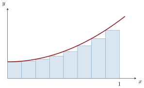
A left Riemann sum with n=8 rectangles: as the mesh shrinks, uniform continuity forces the staircase area toward ∫abf.
Example 15.21
k=1∑nn+k1=n1k=1∑n1+k/n1n→∞∫011+xdx=ln2: a limit invisible to elementary bounds, transparent as a Riemann sum.
Example 15.22(A second Riemann sum, with calibration)
a Riemann sum of the continuousf(x)=(1+x)21 on [0,1]: the limit is
∫01(1+x)2dx=[−1+x1]01=21.
The closing insight: the whole art is the middle line — force the summand into the shape f(nk) at the cost of extracting exactly one factor n1; once the shape is right, the theorem does the analysis and the fundamental theorem does the arithmetic.
Remark 15.23(Where the integral works next)
The chapter’s constructions each have a sequel. Riemann sums return in Chapter 17 as the bridge between series and integrals (comparison of ∑nα1 with ∫tαdt); the integral remainder is the sharpest form of Taylor’s formula in Chapter 16; the sup-based definition is the prototype for the Lebesgue integral of the Year 3 volume, where the same three properties (linearity, monotonicity, a convergence theorem) are rebuilt on a far larger class of functions. And the weekend problem below turns integration by parts into arithmetic: the irrationality of π2.
un=n1∑k=1n1+(k/n)21: a Riemann sum of x↦1+x21 on [0,1], so un→∫011+x2dx=arctan1=4π.
lnvn=n1∑k=1nlnnn+k=n1∑k=1nln(1+nk)→∫01ln(1+x)dx=[(1+x)ln(1+x)−x]01=2ln2−1. Hence vn→e2ln2−1=e4. (Check of the identification: n!nn(2n)!=∏k=1nnn+k.)
Exercise 15.4★
Let f be continuous on [0,1]. Compute limn→∞∫01xnf(x)dx. (Cut [0,1] at 1−δ.)
Solution
Solution of Exercise 15.4.
The limit is 0. Let M=sup∣f∣ and ε∈(0,1). Cut at 1−ε:
∫01xnf≤∫01−εxn∣f∣+∫1−ε1xn∣f∣≤M(1−ε)n+Mε.
Since (1−ε)n→0 (Exercise 11.3), the limsup of the left side is ≤Mε for every ε: the integral tends to 0.
Exercise 15.5★★
(Cauchy–Schwarz) For f,gcontinuous on [a,b], prove
(∫abfg)2≤∫abf2⋅∫abg2,
by expanding ∫ab(f+λg)2≥0 as a quadratic in λ. When is it an equality?
Solution
Solution of Exercise 15.5.
Q(λ)=∫ab(f+λg)2=∫f2+2λ∫fg+λ2∫g2≥0 for all λ. If ∫g2=0, then g=0 (strict positivity, Theorem 15.7 (4)) and the inequality is 0≤0. Otherwise Q is a genuine quadratic, everywhere ≥0: its discriminant is ≤0, i.e. (∫fg)2≤∫f2∫g2.
Equality iff the discriminant vanishes iff Q(λ0)=0 for some λ0, i.e. ∫(f+λ0g)2=0, i.e. (strict positivity again) f=−λ0g: equality holds exactly when f and g are proportional.
Exercise 15.6★★
Let f be continuous on R, T-periodic. Prove that ∫aa+Tf does not depend on a, and that x1∫0xf(t)dt→T1∫0Tf as x→+∞.
Solution
Solution of Exercise 15.6.
Let Φ(a)=∫aa+Tf. By the fundamental theorem (Theorem 15.9), Φ is differentiable with Φ′(a)=f(a+T)−f(a)=0: constant.
Then x1∫0xf=xnT⋅T1∫0Tf+O(x1), and xnT→1: the limit is T1∫0Tf.
Exercise 15.7★★
For fcontinuous on [0,1] with ∫01f=21, prove that f has a fixed point in [0,1]. (Integrate f(x)−x and use strict positivity, Theorem 15.7 (4), through its contrapositive combined with the intermediate value theorem.)
If g never vanished, the intermediate value theorem would force a constant sign (a continuous function on an interval taking both signs vanishes); say g>0. Then, by strict positivity (Theorem 15.7 (4) applied to g>0, giving ∫g>0): contradiction with ∫g=0. So g(c)=0 for some c: f(c)=c.
On (0,2π), 0<sint<1, so sinn+1<sinn and (Wn) is (strictly) decreasing, positive. Sandwiching with the recurrence:
n+1n=Wn−1Wn+1≤WnWn+1≤1⟹WnWn+1→1.
Invariant: an=(n+1)Wn+1Wn satisfies an=an−1 by the recurrence (n+1)Wn+1=nWn−1, so an=a0=1⋅W1W0=2π. Then
nWn2∼(n+1)Wn+1Wn=2π⟹Wn∼2nπ.
Exercise 15.9★★★
(Niven: π is irrational) Suppose π=ba with a,b∈N∗, and set, for n to be chosen,
P(x)=n!xn(a−bx)n,In=∫0πP(x)sinxdx.
Prove that 0<In≤πn!(πa)n, which is <1 for n large.
Prove that P and all its derivatives take integer values at 0 and at π=ba. (Binomial expansion: the coefficients of P times k! are integers for k≥n; and P(π−x)=P(x).)
Set Q=P−P′′+P(4)−… (a finite sum). Check that (Q′sinx−Qcosx)′=Psinx, and deduce that In=Q(π)+Q(0) is an integer.
Conclude.
Solution
Solution of Exercise 15.9.
On (0,π): x>0, a−bx=b(ba−x)=b(π−x)>0 and sinx>0, so the integrand is >0 and In>0 (strict positivity). Bound: on [0,π], x≤π and a−bx≤a, so P≤n!πnan and In≤πn!(πa)n, which tends to 0 (the factorial beats the geometric term: it is the general term of the convergent exponential series, cf. Example 11.12); in particular In<1 for large n.
Expand xn(a−bx)n=∑j=0n(jn)an−j(−b)jxn+j: so P=n!1∑jcjxn+j with integer cj. Then P(k)(0)=0 for k<n (valuation) and, for n≤k≤2n, P(k)(0)=n!k!ck−n, an integer since n!∣k!. Moreover P(π−x)=P(x) (substitute: π−x swaps the factors, using a−b(π−x)=bx), so P(k)(π)=±P(k)(0): integers as well.
With Q=P−P′′+P(4)−… (finite: P has degree 2n): Q+Q′′=P, and
(Q′sinx−Qcosx)′=(Q+Q′′)sinx=Psinx.
Hence In=[Q′sinx−Qcosx]0π=Q(π)+Q(0), a sum of values P(2k) at 0 and π: an integer by (2).
For n large, In is an integer with 0<In<1: impossible. The assumption π=ba fails: π is irrational.
Exercise 15.10★★★
Let f be C1 on [a,b]. Prove the Riemann–Lebesgue-type limit
and each ∫sinλt=λcosλxi−1−cosλxi≤λ2: the second term tends to 0. Hence the limsup is ≤(b−a)ε for every ε: the limit is 0.
Exercise 15.11★★
(Mean value theorem for integrals) Let f,g be continuous on [a,b] with g≥0. Prove that there exists c∈[a,b] with
∫abf(t)g(t)dt=f(c)∫abg(t)dt,
and show by an example that the hypothesis g≥0 cannot be dropped.
Solution
Solution of Exercise 15.11.
Let m=minf and M=maxf, attained by the extreme value theorem. Since g≥0: mg≤fg≤Mg, so by monotonicity
m∫abg≤∫abfg≤M∫abg.
If ∫abg=0: strict positivity (Theorem 15.7 (4)) forces g≡0, both sides vanish, and any c works. Otherwise t=∫g∫fg lies in [m,M]=f([a,b]) (Theorems 13.13 and 13.10), so t=f(c) for some c.
Sign matters: on [−1,1] with f(t)=g(t)=t: ∫fg=∫−11t2=32, while f(c)∫−11tdt=0 for every c.
Exercise 15.12★★★
(Moments force zeros) Let f be continuous on [a,b] with
∫abf(t)tkdt=0for k=0,1,…,n.
Prove that f vanishes at n+1 distinct points of (a,b). (If f changes sign only at z1<⋯<zm with m≤n, integrate f against P(t)=(t−z1)⋯(t−zm) and use strict positivity.)
Solution
Solution of Exercise 15.12.
If f≡0 the claim is vacuous (every point is a zero). So assume f≡0 and suppose it has at most n distinct zeros in (a,b); let z1<⋯<zm (m≤n) be those zeros where fchanges sign (possibly none). Set P(t)=∏i=1m(t−zi) (empty product =1), of degree m≤n. On each subinterval cut by the zi, both f and P have constant sign, and both flip sign when crossing some zi: the product fP has one constant sign on all of (a,b). Being continuous, not identically zero, of constant sign, it has ∫abfP>0 (strict positivity applied to ∣fP∣). But ∫fP is a linear combination of the moments ∫ftk, k≤n, all zero: contradiction. Hence f has at least n+1 distinct zeros in (a,b).
Remark 15.24(Perspectives inside this volume)
Three chapters ahead lean directly on this one. Chapter 16 carries the integral remainder — the sharpest of the three Taylor formulas is an integration by parts iterated n times. Chapter 17 converts the framing of sums by integrals into the decisive test for ∑n−α, and its weekend problem refines that framing into Euler’s constant. Chapter 24 makes the integral geometric: the length of a parametrized arc is ∫x′(t)2+y′(t)2dt, an integral of a continuous function on a segment — precisely the object built here, no improper theory needed. The single most reused fact will be the humblest: ∫f≤(b−a)sup∣f∣, the inequality that turns every pointwise estimate into an integral estimate.
15.6 Problem: The integral irrationality machine
Problem 15.1
Weekend problem — e and π2 are irrational, e to six decimals, and 722>π with proof
One mechanism powers this whole problem: an expression that must be a positive integer, yet is provably smaller than 1, cannot exist. Exercise 15.9 (Niven) ran it once to prove π∈/Q; here we industrialize it. The machine needs three parts: an integrality input (endpoint values of well-chosen polynomials), a smallness input (a factor n!1 crushing the integral), and a bridge (integration by parts) connecting them. We prove that e is irrational and compute it with certified error, prove Legendre’s sharper theorem that π2 is irrational, and end with the most charming integral in analysis: ∫011+x2x4(1−x)4dx=722−π, which brackets π by hand.
Part I — Fuel.
Prove that n!cn→0 for every fixed c>0(beyond n≥2c, each step at least halves the term).
Deduce ∫01(x(1−x))ndx=(2n+1)(n2n)1, and — comparing with the bound x(1−x)≤41 — the estimate (n2n)≥2n+14n, matching (n2n)1/n→4 from Problem 11.1.
Prove the smallness lemma used twice below: for every continuousg>0 on (0,1),
0<∫01(x(1−x))ng(x)dx≤4nsup[0,1]∣g∣.
Part II — e: irrationality, then six decimals. Set An=∫01xnexdx.
Compute A0 and A1, prove the recurrence An=e−nAn−1, and the bounds 0<An≤n+1e.
Show by induction that An=αn+βne with αn,βn∈Z.
Deduce that e is irrational (if e=qp, then qAn is an integer trapped in (0,1) for n large). Compare with the proof of Exercise 11.9: same punchline, different fuel.
Take n=9: bound R9 using e<2.75 (from b2=2.75 in Example 11.12), evaluate the sum, and conclude the certified bracketing 2.7182818≤e≤2.7182823 — six decimals, e≈2.718282, with proof.
Part III — Legendre’s theorem: π2 is irrational. Let f(x)=n!xn(1−x)n, and suppose π2=ba with a,b∈N∗.
Show f(1−x)=f(x) and 0<f≤4nn!1 on (0,1).
Show that f(k)(0) and f(k)(1) are integers for every k≥0(expand xn(1−x)n with integer coefficients; n!k!∈Z for k≥n; then use the symmetry).
Define
G=bnk=0∑n(−1)kπ2n−2kf(2k).
Show that G(0) and G(1) are integers (each bnπ2n−2k=an−kbk).
Verify the telescoping G′′+π2G=bnπ2n+2f=π2anf, then
dxd(G′(x)sinπx−πG(x)cosπx)=π2anf(x)sinπx.
Integrate over [0,1] and conclude
πan∫01f(x)sin(πx)dx=G(0)+G(1)∈Z,
a positive integer bounded by 4nn!πan.
Conclude with question 1 that π2 is irrational (Legendre, 1794), and that this strengthens Exercise 15.9: why does the irrationality of π2 imply that of π, and not conversely?
Part IV — Understanding the machine.
Locate the two opposing forces (integrality of endpoint data; analytic smallness of the integral) and the bridge, in Parts II and III. Then explain why the factor n!1 in f is the crux: if it is removed, integrality survives, but which inequality dies, and for which claimed fractions ba does the proof then fail?
Effectivity: suppose someone claims π2=ba with a≤10. Show that the contradiction already lands at n=7: compute π(10/4)7/7!≈0.38<1. The machine does not merely refute; it refutes by a fixed, computable stage.
Sanity check the bridge unconditionally: prove by two integrations by parts that
∫01x(1−x)sin(πx)dx=π34,
and reconcile with question 14 at n=1 (keep π2 symbolic: the telescoped identity reads π3∫01f1sinπx=−(f1′′(0)+f1′′(1))=4).
What makes ex and sinπx eligible as the machine’s kernels? Identify the property (each satisfies a linear differential equation with constant coefficients, so repeated integration by parts cycles back to the start), and name the frontier: the same machine, refined by Hermite and Lindemann, proves e and πtranscendental — beyond this volume.
The integrand is positive: conclude π<722. Then, bounding 1+x21 between 21 and 1 and using ∫01(x(1−x))4=6301 (question 3), prove
722−6301≤π≤722−12601,
i.e. 3.14126≤π≤3.14207: two correct decimals, by hand.
Generalize: dividing x4m(1−x)4m by 1+x2, show the remainder is the constant (−4)m(work modulo x2+1: (1−x)2≡−2x), deduce rationals rm with
∣π−rm∣≤41−5m,
and check that m=1 reproduces question 20–21.
Confront these rationals with the approximation theory of Problem 14.1: compute π−722≈1.26⋅10−3 against the Dirichlet guarantee 491, and quote π−113355≈2.7⋅10−7 against 11321≈7.8⋅10−5: exceptionally good rational approximations exist for π — consistent, since π is not known to be badly approximable.
(The integer trap, abstracted) Prove the lemma that unifies everything: if x∈R and there exist integers an,bn with 0<∣an+bnx∣→0, then x is irrational. List its instances in this problem, in Exercise 15.9, in Exercise 11.9, and in Problem 14.1.
Synthesis, one sentence each: (i) the machine’s three parts and where each lives in the toolbox of this chapter; (ii) what the integral contributes that the mean value theorem of Problem 14.1 could not; (iii) the inventory of results extracted (two irrationalities, one six-decimal constant, one bracketing of π, one binomial bound); (iv) the frontier (Hermite, Lindemann; and the same trap, run on ζ(2) and ζ(3), in twentieth-century arithmetic).
Solution
Solution of Problem 15.1.
1. Let N=⌈2c⌉. For n≥N: cn/n!cn+1/(n+1)!=n+1c≤21, so 0<n!cn≤N!cN2−(n−N)→0: squeeze.
2. Fix k; induction on m. For m=0: ∫01xk=k+11=(k+1)!k!0!. Step, by parts (u=(1−x)m, v′=xk):
3.k=m=n: ∫01(x(1−x))n=(2n+1)!(n!)2=(2n+1)(n2n)1. Since x(1−x)≤41 on [0,1], the integral is ≤4−n, whence (n2n)≥2n+14n — consistent with (n2n)1/n→4 (Problem 11.1).
4. The integrand is continuous, ≥0, and positive on (0,1), hence not identically zero: its integral is >0 (Theorem 15.7 (4)). Upper bound: (x(1−x))n≤4−n and g≤sup∣g∣, then monotonicity.
5.A0=e−1; A1=[xex]01−∫01ex=e−(e−1)=1. By parts: An=[xnex]01−n∫01xn−1ex=e−nAn−1. Bounds: the integrand is positive, so An>0; and ex≤e gives An≤e∫01xn=n+1e.
6.A0=−1+1⋅e. If An−1=αn−1+βn−1e with integer entries, then
7. If e=qp: qAn=qαn+pβn∈Z, and 0<qAn≤n+1qe<1 for n large: an integer strictly between 0 and 1 — impossible. So e∈/Q. In Exercise 11.9 the trapped integer was q!qp−q!aq; here it is qAn: same trap, integral fuel.
8.n=0: R0=∫01et=e−1, so e=1+R0. By parts (u=et, v=−n+1(1−t)n+1):
so the formula propagates from n to n+1. Bounds: 1≤et≤e on [0,1] and ∫01(1−t)n=n+11 give (n+1)!1≤Rn≤(n+1)!e.
9.∑k=09k!1=362880986410=2.71828152…, and
10!1=2.76⋅10−7≤R9≤10!2.75=7.58⋅10−7,
so 2.7182818≤e≤2.7182823: with proof, e=2.718282 to six decimals (true value 2.7182818…).
10.f(1−x)=n!(1−x)nxn=f(x). On (0,1): 0<x(1−x)≤41, so 0<f≤4nn!1.
11.xn(1−x)n=∑j=0n(−1)j(jn)xn+j, so f=n!1∑jcjxn+j with cj∈Z. Hence f(k)(0)=0 for k<n or k>2n, and for n≤k≤2n: f(k)(0)=n!k!ck−n, an integer because n!∣k!. The symmetry gives f(k)(1)=(−1)kf(k)(0)∈Z.
12.bnπ2n−2k=bn(ba)n−k=an−kbk∈Z, so G(0)=∑k(−1)kan−kbkf(2k)(0) and likewise G(1) are integers by question 11.
13. In π2G+G′′, the term k of π2G carries π2n−2k+2f(2k) and the term j=k−1 of G′′ carries (−1)k−1π2n−2k+2f(2k): everything cancels except k=0 in the first sum and j=n in the second, i.e.
G′′+π2G=bn(π2n+2f+(−1)nf(2n+2))=bnπ2n+2f=π2anf
(f has degree 2n, so f(2n+2)=0; and bnπ2n=an). Then
so πan∫01fsinπx=G(0)+G(1)∈Z. On (0,1), f>0 and sinπx>0: the left side is positive, so G(0)+G(1)≥1; and sin≤1 with question 10 bounds it by 4nn!πan.
15. By question 1 (with c=4a), 4nn!πan→0: for large n it is <1, contradicting G(0)+G(1)≥1. So no fraction ba equals π2: Legendre’s theorem. If π were rational, π2 would be too: so π∈/Q — and the implication only runs this way (2 is irrational with rational square), which is why π2∈/Q is strictly stronger than Exercise 15.9.
16. Integrality: questions 11–12 (endpoint derivatives); smallness: questions 10 and 1; bridge: questions 13–14 (the telescoped double integration by parts). Without n!1, the endpoint data remain integers (even more easily), but the bound becomes 4nπan, which tends to 0 only when a<4 — and every candidate has a=bπ2>9. The factorial is exactly what outruns the geometric growth an: no factorial, no theorem.
17. For a≤10, the integer G(0)+G(1) is positive and at most π(10/4)n/n!. At n=7: 2.57=610.35…, so the bound is 5040π×610.35≈0.38<1 (at n=6 it is still 1.07): the contradiction lands at the seventh stage, explicitly.
(the bracket terms vanish: x(1−x) at 0,1, and sinπx at 0,1). Symbolically, the n=1 telescope (no assumption on π) reads π3∫01f1sinπx=−(f1′′(0)+f1′′(1)) with f1=x(1−x), f1′′=−2: right side 4 — the two computations agree.
19.ex solves y′=y and sinπx solves y′′=−π2y: linear equations with constant coefficients, so integration by parts cycles the kernel back to itself and keeps all boundary data inside Z+Ze (resp. integer polynomials in π2). That closure property is what the machine needs. Refined with kernels adapted to several points at once, the same mechanism yields Hermite’s theorem (e transcendental, 1873) and Lindemann’s (π transcendental, 1882) — beyond this volume.
20.Polynomial division (or multiply back and check):
x4(1−x)4=(x6−4x5+5x4−4x2+4)(1+x2)−4.
Integrating the displayed identity divided by 1+x2:
21. The integrand is continuous, positive on (0,1): the integral is >0, so π<722. Moreover 21≤1+x21≤1 on [0,1] and ∫01(x(1−x))4=9!(4!)2=6301 (question 3):
22. Modulo x2+1: x2≡−1, so x4m=(x2)2m≡1 and (1−x)2=1−2x+x2≡−2x, hence (1−x)4m≡(−2x)2m=4m(x2)m≡(−4)m: the remainder is the constant (−4)m, and the quotient Qm has integer coefficients (division by a monic integer polynomial). Dividing the identity by 1+x2 and integrating:
Solving for π: with rm=(−1)m+141−msm∈Q, ∣π−rm∣=41−mJm≤41−m⋅4−4m=41−5m. For m=1: s1=722, r1=722, bound 4−4=2561 — questions 20–21 again.
23.π−722=722−π≈1.26⋅10−3, sixteen times better than the order-2 benchmark 721≈2.0⋅10−2 guaranteed by Dirichlet (Problem 14.1, question 4); and π−113355≈2.7⋅10−7 beats 11321≈7.8⋅10−5 by a factor ≈300. No contradiction with anything proved: Liouville inequalities lower-bound approximation errors only for algebraic numbers, and no such bound for π is available at this level — π is free to be approximated spectacularly well.
24. Lemma: suppose x=qp and 0<∣an+bnx∣→0. Then ∣an+bnx∣=q∣qan+pbn∣, with qan+pbn a nonzero integer (nonzero because the absolute value is >0): so ∣an+bnx∣≥q1 for every n, contradicting the convergence to 0. Instances: question 7 (x=e, an=αn, bn=βn); Exercise 11.9 (x=e again, with aq=−q!∑k≤qk!1, bq=q!); and Problem 14.1, question 1, is its geometric form. In Part III and in Exercise 15.9 the trap runs inside the contradiction: assuming rationality converts an expression into an integer, which the analysis then squeezes into (0,1) — the same principle, transposed.
25. (i) Integrality lives in the endpoint calculus of polynomials (questions 6, 11–12), smallness in the bounds sup-monotonicity gives (questions 4, 10), the bridge in integration by parts (questions 8, 13–14) — all three are theorems of this chapter. (ii) The integral supplies what the mean value theorem could not: an exact identity between the analytic object and the arithmetic data (equality, not just an inequality with an unknown c), which is why the machine reaches π2 while Problem 14.1 reached only approximation exponents. (iii) Extracted: e∈/Q, π2∈/Q (hence π∈/Q), e=2.718282 certified, 722−6301≤π≤722−12601, and (n2n)≥2n+14n. (iv) Frontier: Hermite and Lindemann push the same machine to transcendence; and Apéry (1979) ran the integer trap on ζ(3) — the machine is still producing twentieth-century mathematics.