University Mathematics — Year 1 · Bachelor Year 1

18Vector Spaces

Linear algebra begins here: the axioms of vector spaces isolate what $\R^2$ , $\R^3$ , polynomial spaces and function spaces have in common — one can add, and scale. Two chapters build the theory (Chapter 19 adds dimension); the language they set up — span, free family, basis, direct sum — is the daily bread of every chapter after them. Throughout, $K$ denotes $\R$ or $\C$ (scalars).

18.1 Definition and examples

Definition 18.1 (Vector space)

A $K$ -vector space is a set $E$ with an addition making $(E, +)$ an abelian group (zero written $0_E$ or $0$ ), and a scalar multiplication $K \times E \to E$ such that, for all $\lambda, \mu \in K$ and $x, y \in E$ :

\lambda(x + y) = \lambda x + \lambda y,\quad (\lambda + \mu) x = \lambda x + \mu x,\quad \lambda(\mu x) = (\lambda\mu) x,\quad 1\,x = x .

Consequences: $0\,x = 0_E$ , $\lambda\,0_E = 0_E$ , $(-1)x = -x$ , and $\lambda x = 0_E \implies \lambda = 0$ or $x = 0_E$ (multiply by $\lambda^{-1}$ ).

Proof of the consequences. For $0\,x = 0_E$ : from $(0 + 0)x = 0x + 0x$ and $(0+0)x = 0x$ , cancel $0x$ in the group $(E, +)$ . For $\lambda\,0_E$ : same trick on $\lambda(0_E + 0_E)$ . For $(-1)x$ : add $x$ ,

x + (-1)x = 1\,x + (-1)x = \bigl(1 + (-1)\bigr)x = 0\,x = 0_E ,

so $(-1)x$ is the additive inverse of $x$ . Finally if $\lambda x = 0_E$ with $\lambda \neq 0$ : multiply by $\lambda^{-1}$ (the scalars form a field) and use the two axioms $\lambda^{-1}(\lambda x) = (\lambda^{-1}\lambda)x = 1x = x$ together with $\lambda^{-1}0_E = 0_E$ : $x = 0_E$ . Small as they are, these four rules are used silently on every page that follows — and the last one is exactly where fields are needed: over the scalars $\Z$ , the “space” $\Z/2\Z$ would violate it with $2\,x = 0$ . ∎

Example 18.2

$K^n$ (coordinatewise operations); the polynomials $K[X]$ ; the functions $\mathcal{F}(A, K)$ from any set $A$ to $K$ (pointwise operations) — containing continuous functions, sequences $\mathcal{F}(\N, \R)$ , etc.; $\C$ as an $\R$ -vector space. In each case the axioms are inherited from those of $K$ .

Definition 18.3 (Subspace)

$F \subseteq E$ is a subspace when $0_E \in F$ and $F$ is stable under addition and scalar multiplication — equivalently:

F \neq \emptyset \qquad\text{and}\qquad \forall x, y \in F,\ \forall \lambda \in K,\quad x + \lambda y \in F .

A subspace is itself a vector space. Any intersection of subspaces is a subspace; a union almost never is (same proof as Exercise 7.6).

Example 18.4

In $\mathcal{F}(\R, \R)$ : the continuous functions, the differentiable ones, the polynomials of degree $\leq n$ (written $K_n[X]$ inside $K[X]$ ), the solutions of a homogeneous linear differential equation (Theorem 5.10 said just that). Non-examples: $\{f : f(0) = 1\}$ (no zero), degree exactly $n$ (not stable under addition).

Example 18.5 (Subspace or not: four verdicts, argued)

In the space of real sequences:

$\{u : u \text{ bounded}\}$ is a subspace: $0$ is bounded, and if $\abs{u_n} \leq M$ , $\abs{v_n} \leq M'$ , then $\abs{u_n + \lambda v_n} \leq M + \abs\lambda M'$ .
$\{u : u_n \to 1\}$ is not: the zero sequence is missing (and the sum of two members tends to $2$ ).
$\{u : u \text{ monotone}\}$ is not: $u_n = n$ and $v_n = -n + (-1)^n$ are monotone, their sum $(-1)^n$ is not; stability under addition is the axiom that fails, even though the set contains $0$ and all scalar multiples of its members.
$\{u : u_{n+1} = u_n^2\}$ is not: it contains $0$ but $2u$ escapes as soon as $u$ is a nonzero member ( $2u_{n+1} \neq (2u_n)^2$ in general) — squaring is the nonlinearity.

The working order is always the same: test $0$ first (cheapest), then stability — and to refute, one explicit counterexample pair beats any amount of doubt.

18.2 Span, sums, direct sums

Definition 18.6 (Linear combinations, span)

A linear combination of the family $(x_1, \dots, x_p)$ of vectors of $E$ is any $\lambda_1 x_1 + \dots + \lambda_p x_p$ ( $\lambda_i \in K$ ). The set of all of them is the span $\operatorname{Vect}(x_1, \dots, x_p)$ : it is a subspace, the smallest one containing the family.

Proof of the two assertions. Stability: a sum of two linear combinations $\sum\lambda_i x_i + \sum\mu_i x_i = \sum(\lambda_i + \mu_i)x_i$ is again one, and so is a scalar multiple $\mu\sum\lambda_i x_i = \sum(\mu\lambda_i) x_i$ ; the zero combination shows $0$ belongs: the span is a subspace. Minimality: let $H$ be any subspace containing $x_1, \dots, x_p$ . By stability under scalar multiplication each $\lambda_i x_i \in H$ , and by stability under addition their sum lies in $H$ : every linear combination belongs to $H$ , i.e. $\operatorname{Vect}(x_1, \dots, x_p) \subseteq H$ . So the span is contained in every subspace containing the family: it is the smallest one. ∎

Definition 18.7 (Sum, direct sum)

For subspaces $F, G$ of $E$ :

F + G = \{\,u + v : u \in F,\ v \in G\,\}

is a subspace (the smallest containing $F \cup G$ ). The sum is direct, written $F \oplus G$ , when every element of $F + G$ decomposes uniquely as $u + v$ ; equivalently (see below) when $F \cap G = \{0\}$ . When $E = F \oplus G$ , the subspaces are supplementary in $E$ .

Example 18.8 (A sum of two lines)

In $\R^3$ , let $F = \operatorname{Vect}\bigl((1,0,1)\bigr)$ and $G = \operatorname{Vect}\bigl((0,1,1)\bigr)$ . Their sum is

F + G = \{\,a(1,0,1) + b(0,1,1)\,\} = \{(a,\ b,\ a + b)\} = \{(x, y, z) : z = x + y\},

the plane through the origin containing both lines. It is strictly bigger than the union $F \cup G$ (the mere cross of the two lines): the vector $(1, 1, 2) = (1,0,1) + (0,1,1)$ lies in the sum but on neither line. And $F \cap G = \{0\}$ (a common vector requires $a(1,0,1) = b(0,1,1)$ , whose first two coordinates force $a = b = 0$ ): the sum is direct, and $F \oplus G$ is exactly that plane.

Proposition 18.9

$F + G$ is direct if and only if $F \cap G = \{0\}$ .

Proof. If some $w \neq 0$ lies in $F \cap G$ : $w = w + 0 = 0 + w$ are two decompositions of $w$ . Conversely, if $u + v = u' + v'$ with $u, u' \in F$ , $v, v' \in G$ , then $u - u' = v' - v$ belongs to $F \cap G = \{0\}$ : decompositions are unique. ∎

Method 18.10 (Proving $E = F \oplus G$ )

Two things to check, each with its standard opening move.

Trivial intersection. Take $x \in F \cap G$ , write out both membership conditions, and squeeze $x = 0$ . (Never argue by picture: cf. the pitfalls below.)
Sum is everything. Take an arbitrary $x \in E$ and produce the decomposition $x = f + g$ — either by guessing $f$ from the target ( $f$ must satisfy the defining property of $F$ , which usually dictates its formula) or by solving the linear system expressing $x$ against generators of $F$ and $G$ .

When the decomposition formula is guessed, uniqueness is automatic from step 1; when only existence is unclear, step 2 is where the work lives. The two examples below run the method: for even/odd functions the formula for $f$ is forced by evaluating the desired identity at $x$ and $-x$ ; for polynomials vanishing at a point, by evaluating at $a$ .

Example 18.11

In $\mathcal{F}(\R, \R)$ , the even functions $\mathcal{P}$ and the odd functions $\mathcal{I}$ are supplementary: any $f$ writes

f(x) = \underbrace{\frac{f(x) + f(-x)}{2}}_{\text{even}} + \underbrace{\frac{f(x) - f(-x)}{2}}_{\text{odd}},

and a function both even and odd is zero. (Applied to $\exp$ , this is the pair $(\cosh, \sinh)$ of Chapter 4.)

Example 18.12 (A supplementary pair in $K_n[X]$ )

Fix $a \in K$ and set $F = \{P \in K_n[X] : P(a) = 0\}$ , $G = \operatorname{Vect}(1)$ (the constants). Then $K_n[X] = F \oplus G$ . Indeed $F \cap G$ consists of the constants vanishing at $a$ , i.e. $\{0\}$ ; and every $P$ decomposes as

P = \underbrace{\bigl(P - P(a)\bigr)}_{\in F} + \underbrace{P(a)}_{\in G} .

The decomposition is worth memorizing: subtracting the value at a point is the standard way to project onto “functions vanishing at $a$ ”. Note that $F$ is a large subspace and $G$ a small one; a supplementary pair need not be balanced in any sense.

Example 18.13 (A supplementary subspace is never unique)

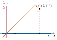
In $\R^2$ , let $F = \operatorname{Vect}\bigl((1,0)\bigr)$ (the $x$ -axis). Both $G = \operatorname{Vect}\bigl((0,1)\bigr)$ and $G' = \operatorname{Vect}\bigl((1,1)\bigr)$ are supplementary to $F$ : each meets $F$ only at $0$ , and each pair sums to $\R^2$ . The decompositions of a same vector differ:

(2,\ 1.5) = \underbrace{(2, 0)}_{\in F} + \underbrace{(0, 1.5)}_{\in G} = \underbrace{(0.5,\ 0)}_{\in F} + \underbrace{(1.5,\ 1.5)}_{\in G'} .

In fact every line other than $F$ itself is a supplementary of $F$ in $\R^2$ : supplementaries are plentiful, and speaking of “the” supplementary is meaningless until an extra structure (an inner product, Chapter 23) singles one out.

Two decompositions of the same point of ℝ2 along F (the x-axis): with supplementary G (vertical drop) and with supplementary G' (oblique drop). The F-components differ: a projection depends on the direction of descent. — Two decompositions of the same point of $\R^2$ along $F$ (the $x$ -axis): with supplementary $G$ (vertical drop) and with supplementary $G'$ (oblique drop). The $F$ -components differ: a projection depends on the direction of descent.

18.3 Free families, generating families, bases

Definition 18.14

A family $(x_1, \dots, x_p)$ of vectors of $E$ is:

generating (of $E$ ) when $\operatorname{Vect}(x_1,\dots,x_p) = E$ ;
free (its vectors linearly independent) when

$\lambda_1 x_1 + \dots + \lambda_p x_p = 0 \implies \lambda_1 = \dots = \lambda_p = 0 ;$

otherwise linked;
a basis when it is free and generating.

Proposition 18.15 (Coordinates)

$(e_1, \dots, e_n)$ is a basis of $E$ if and only if every $x \in E$ is uniquely a combination $x = \lambda_1 e_1 + \dots + \lambda_n e_n$ ; the scalars $\lambda_i$ are the coordinates of $x$ in the basis.

Proof. Generating $=$ existence of the decomposition. Uniqueness $=$ freeness: two decompositions of the same $x$ differ by a combination equal to $0$ ; freeness forces all its coefficients — the differences of coordinates — to vanish. Conversely, a nontrivial null combination gives the two decompositions $0 = \sum \lambda_i e_i = \sum 0\,e_i$ . ∎

Example 18.16

The canonical basis of $K^n$ : $e_i = (0, \dots, 1, \dots, 0)$ ( $1$ in slot $i$ ). The monomials $(1, X, X^2, \dots, X^n)$ : a basis of $K_n[X]$ (freeness: a null combination is the zero polynomial, so all coefficients vanish, Definition 8.1). In $\C$ over $\R$ : the basis $(1, \iu)$ .

Remark 18.17 (Coordinates are a team effort)

The first coordinate of $x$ in a basis $(e_1, \dots, e_n)$ depends on all the basis vectors, not just $e_1$ . In $\R^2$ : the vector $(3, 1)$ has first coordinate $3$ in the canonical basis, but first coordinate $2$ in the basis $\bigl((1,0), (1,1)\bigr)$ — solve $(3,1) = a(1,0) + b(1,1)$ : $b = 1$ , $a = 2$ . Changing one basis vector reshuffles every coordinate; Chapter 21 will package this reshuffling into the change-of-basis matrix.

Example 18.18 (Testing a candidate basis, start to finish)

Is $\mathcal{F} = (1 + X,\ 1 + X^2,\ X + X^2)$ a basis of $\R_2[X]$ ? Write $u_1, u_2, u_3$ for the three polynomials. Freeness: a null combination $a\,u_1 + b\,u_2 + c\,u_3 = 0$ gives, coefficient by coefficient,

a + b = 0, \qquad a + c = 0, \qquad b + c = 0 ;

subtracting the first two, $b = c$ , then the third gives $2b = 0$ : $a = b = c = 0$ , free. Generating: instead of solving three systems, notice the symmetric combination

u_1 + u_2 - u_3 = (1 + X) + (1 + X^2) - (X + X^2) = 2 ,

so $1 = \frac12(u_1 + u_2 - u_3)$ ; then

X = u_1 - 1 = \tfrac12\bigl(u_1 - u_2 + u_3\bigr), \qquad X^2 = u_2 - 1 = \tfrac12\bigl(-u_1 + u_2 + u_3\bigr).

The monomials lie in the span, so everything does: $\mathcal{F}$ is a basis. As a bonus, assembling the three displays gives the coordinates of any $P = \alpha + \beta X + \gamma X^2$ :

P = \frac{\alpha + \beta - \gamma}{2}\,u_1 + \frac{\alpha - \beta + \gamma}{2}\,u_2 + \frac{-\alpha + \beta + \gamma}{2}\,u_3 .

(Sanity check with $P = X$ : coordinates $\bigl(\frac12, -\frac12, \frac12\bigr)$ , as found above.) Two lessons: symmetry in the family usually hides a shortcut combination; and once dimension is available (Chapter 19), the whole generating half of this work will come free of charge — three free vectors of a $3$ -dimensional space always form a basis.

Proposition 18.19 (Useful freeness criteria)

A family of nonzero polynomials of pairwise distinct degrees is free.
Adding a vector to a free family keeps it free if and only if the vector is outside the span of the family.
Any subfamily of a free family is free; any family containing a generating family is generating.

Proof. (1) In a null combination, look at the highest degree present: its coefficient must vanish (nothing cancels that degree), and cascade down.

(2) If $x \in \operatorname{Vect}(x_1, \dots, x_p)$ , the relation $x - \sum\lambda_i x_i = 0$ is nontrivial. Conversely, a nontrivial null combination of $(x_1, \dots, x_p, x)$ must involve $x$ with a nonzero coefficient (else it contradicts freeness of the small family), and solving for $x$ puts it in the span.

(3) Subfamily: a null combination of the subfamily is one of the whole family with the missing coefficients set to $0$ ; freeness of the big family kills all of them. Superfamily: every vector of $E$ is already a combination of the generating part; give the extra vectors the coefficient $0$ . ∎

Example 18.20 (The staircase principle)

Let $P_0, P_1, \dots, P_n \in K_n[X]$ with $\deg P_k = k$ for each $k$ (a “staircase” of degrees). Then $(P_0, \dots, P_n)$ is a basis of $K_n[X]$ . Freeness is Proposition 18.19 (1). For the generating property, argue by finite descent on the degree: let $Q \in K_n[X]$ , $Q \neq 0$ , of degree $d$ , with leading coefficient $a$ , and let $b \neq 0$ be the leading coefficient of $P_d$ . Then $Q - \frac ab P_d$ has degree $< d$ (the top terms cancel); replacing $Q$ by this difference and iterating, after at most $n + 1$ steps one reaches the zero polynomial, and unwinding the subtractions expresses $Q$ as a combination of the $P_k$ . Two staircases already met: the shifted powers $\bigl((X-a)^k\bigr)_{0 \leq k \leq n}$ (Exercise 18.4), and the Newton products $\bigl((X - x_0)(X - x_1)\cdots(X - x_{k-1})\bigr)_{0 \leq k \leq n}$ , put to work in the weekend problem.

Example 18.21 (Freeness in function spaces)

In $\mathcal{F}(\R,\R)$ , the family $(\eu^{a_1 x}, \dots, \eu^{a_p x})$ with $a_1 < \dots < a_p$ is free: divide a null combination by $\eu^{a_p x}$ and let $x \to +\infty$ ; the last coefficient dies, and one cascades down (Exercise 18.8 details this and variants). Freeness of functions is proved by evaluating: at well-chosen points, at infinity, or after differentiating.

Example 18.22 (A hidden relation shrinks a span)

In $\mathcal{F}(\R, \R)$ , what is $\operatorname{Vect}(1,\ \cos^2,\ \sin^2)$ ? The identity $\cos^2 + \sin^2 = 1$ is a nontrivial null combination

1\cdot\mathbf{1} + (-1)\cos^2 + (-1)\sin^2 = 0 :

the family is linked, and the span is already generated by $(1, \cos^2)$ alone ( $\sin^2 = 1 - \cos^2$ ). That smaller family is free: $a + b\cos^2 x = 0$ for all $x$ gives, at $x = 0$ and $x = \frac\pi2$ : $a + b = 0$ and $a = 0$ . So the span is a plane inside the function space — and it also contains $\cos 2x = 2\cos^2 x - 1$ : linear-looking families of trigonometric functions routinely collapse under identities, which is why freeness must be proved, never assumed from the list’s length.

Remark 18.23 (Common pitfalls)

Four classical traps. Pairwise is not enough: in $\R^2$ , the vectors $(1,0)$ , $(0,1)$ , $(1,1)$ are pairwise non-proportional, yet linked — freeness is a property of the whole family, tested by one global combination, never two by two. The zero vector poisons everything: any family containing $0$ is linked ( $1\cdot 0 = 0$ is a nontrivial relation), however innocent the other vectors. Union is not sum: $F \cup G$ is almost never a subspace (Definition 18.3); the smallest subspace containing both is $F + G$ , usually much bigger than the union — in $\R^2$ , two distinct lines have union a cross, sum the whole plane. Direct requires trivial intersection, not disjointness: two subspaces are never disjoint (both contain $0$ ); the correct condition is $F \cap G = \{0\}$ , and it must be proved, not read off a drawing — cf. Example 18.13, where many different $G$ work. Freeness depends on the scalars: the pair $(1, \iu)$ is free in $\C$ seen as an $\R$ -vector space, but linked in $\C$ seen as a $\C$ -vector space ( $\iu\cdot 1 + (-1)\cdot\iu = 0$ ). Always know which field is acting before declaring a family free — the weekend problem of Chapter 19 turns exactly this sensitivity into irrationality proofs.

Remark 18.24 (Where this language goes)

Everything after this chapter speaks the language set up here. Chapter 19 counts basis vectors and turns “free” and “generating” into inequalities on a single integer, the dimension. Chapter 20 studies the maps compatible with the two operations; direct sums become projectors there. Chapter 21 encodes vectors by their coordinates in a basis — Proposition 18.15 is the licence for that encoding — and Chapter 23 adds lengths and angles on top of the linear structure. In the Year 2 volume the same axioms, verbatim, run over arbitrary fields and in infinite dimension; nothing in this chapter used finiteness anywhere.

Remark 18.25 (Three threads to follow through Book 3)

Watch three specific ideas of this chapter grow. The staircase principle (Example 18.20) reappears as the Newton basis in this chapter’s weekend problem, as the binomial basis $(B_k)$ there, and as the polynomial alternant trick in the weekend problem of Chapter 22: one lemma, three determinant-free dividends. Evaluation as a freeness test (Example 18.21) becomes the interpolation isomorphism of Chapter 20, then the Vandermonde criterion of Chapter 22, then the Gram test of Chapter 23: the same reflex, sharpened three times. Direct sums (Definition 18.7) become projectors in Chapter 20, orthogonal splittings $E = F \oplus F^\perp$ in Chapter 23, and the explained-plus-residual decomposition of least squares in the weekend problem of Chapter 25. Very little of this book is not, at bottom, one of these three ideas wearing new clothes.

18.4 Exercises

Exercise 18.1 ★

Which of the following are subspaces?

$\{(x, y, z) \in \R^3 : x + 2y - z = 0\}$ ;
$\{(x, y, z) \in \R^3 : x + 2y - z = 1\}$ ;
$\{(x, y) \in \R^2 : xy \geq 0\}$ ;
$\{P \in \R[X] : P(1) = 0\}$ ;
$\{f \in \mathcal{F}(\R,\R) : f \text{ bounded}\}$ .

Solution

Solution of Exercise 18.1.

Yes: contains $0$ , and the defining equation is linear (stable under $x + \lambda y$ ).
No: does not contain $(0,0,0)$ .
No: $(1, 0)$ and $(0, -1)$ belong ( $xy = 0$ ), their sum $(1, -1)$ does not ( $xy = -1 < 0$ ).
Yes: $0$ vanishes at $1$ ; $(P + \lambda Q)(1) = P(1) + \lambda Q(1) = 0$ .
Yes: the zero function is bounded; if $\abs f \leq M$ and $\abs g \leq M'$ , then $\abs{f + \lambda g} \leq M + \abs\lambda M'$ .

Exercise 18.2 ★

In $\R^3$ , is $(1, 2, 1)$ in $\operatorname{Vect}\bigl((1,0,1),\, (1,1,0)\bigr)$ ? And $(2, 1, 1)$ ? Describe $\operatorname{Vect}\bigl((1,0,1),(1,1,0)\bigr)$ by an equation.

Solution

Solution of Exercise 18.2.

$(1,2,1) = a(1,0,1) + b(1,1,0)$ requires $a + b = 1$ , $b = 2$ , $a = 1$ : incompatible ( $a + b = 3 \neq 1$ ): not in the span. $(2,1,1) = a(1,0,1) + b(1,1,0)$ : $b = 1$ , $a = 1$ , $a + b = 2$ : consistent, so $(2,1,1) = (1,0,1) + (1,1,0)$ , in the span.

Equation: $(x, y, z) = (a + b, b, a)$ means $x = y + z$ : the span is the plane $\{x - y - z = 0\}$ .

Exercise 18.3 ★

Decide freeness in $\R^3$ : $\;\bigl((1,1,0), (1,0,1), (0,1,1)\bigr)$ ; $\;\bigl((1,2,3), (2,4,6)\bigr)$ ; $\;\bigl((1,0,0), (1,1,0), (1,1,1), (0,1,1)\bigr)$ .

Solution

Solution of Exercise 18.3.

First family: $\lambda(1,1,0) + \mu(1,0,1) + \nu(0,1,1) = 0$ gives $\lambda + \mu = 0$ , $\lambda + \nu = 0$ , $\mu + \nu = 0$ : adding, $2(\lambda + \mu + \nu) = 0$ , and subtracting each equation, $\lambda = \mu = \nu = 0$ : free.

Second: $(2,4,6) = 2(1,2,3)$ : linked.

Third: four vectors in $\R^3$ — necessarily linked once dimension is available (Chapter 19); directly: $(0,1,1) = -(1,0,0) + 0\cdot(1,1,0) + (1,1,1)$ , indeed $(-1,0,0) + (1,1,1) = (0,1,1)$ : a nontrivial relation.

Exercise 18.4 ★

Prove that $(1, X - 1, (X-1)^2, (X-1)^3)$ is a basis of $\R_3[X]$ , and give the coordinates of $X^3$ in it. (Taylor at $1$ !)

Solution

Solution of Exercise 18.4.

Polynomials $1, (X-1), (X-1)^2, (X-1)^3$ have distinct degrees $0, 1, 2, 3$ : free (Proposition 18.19 (1)); four free vectors generating (every $P \in \R_3[X]$ expands in powers of $X - 1$ , e.g. by Taylor for polynomials, cf. the proof of Proposition 8.11): a basis. For $X^3$ , Taylor at $1$ : $P = X^3$ , $P(1) = 1$ , $P'(1) = 3$ , $P''(1) = 6$ , $P'''(1) = 6$ :

X^3 = 1 + 3(X - 1) + 3(X-1)^2 + (X-1)^3 ,

coordinates $(1, 3, 3, 1)$ (Pascal’s row, as expected from $X^3 = ((X-1)+1)^3$ ).

Exercise 18.5 ★★

In $\R^4$ , let $F = \{(x,y,z,t) : x = y = z\}$ and $G = \{(x,y,z,t) : x = t = 0\}$ . Prove that $F \oplus G = \R^4$ , and decompose $(1,2,3,4)$ accordingly.

Solution

Solution of Exercise 18.5.

$F \cap G$ : the conditions $x = y = z$ and $x = t = 0$ together give $x = 0$ , hence $y = z = 0$ , and $t = 0$ : the intersection is $\{0\}$ . Sum: given $(x,y,z,t)$ , seek $(a,a,a,b) \in F$ and $(0,c,d,0) \in G$ summing to it: $a = x$ , $b = t$ , $c = y - x$ , $d = z - x$ : always possible. So $\R^4 = F \oplus G$ , and

(1,2,3,4) = (1,1,1,4) + (0,1,2,0) .

Exercise 18.6 ★★

In the space of sequences, let $F$ be the set of convergent sequences and $G = \operatorname{Vect}(u)$ where $u_n = (-1)^n$ . Prove that $F \cap G = \{0\}$ . Is $F + G$ the whole space of sequences?

Solution

Solution of Exercise 18.6.

An element of $G$ is $\lambda u$ ; if it converges, then (as $\lambda u_n = \lambda(-1)^n$ has the two subsequential limits $\pm \lambda$ ) necessarily $\lambda = 0$ : $F \cap G = \{0\}$ .

$F + G$ is not everything: it consists of sequences of the form $c_n + \lambda(-1)^n$ with $(c_n)$ convergent. The sequence $v_n = n$ is not of this form ( $v_n - \lambda(-1)^n$ is unbounded, never convergent). So $F \oplus G \subsetneq$ (space of all sequences).

Exercise 18.7 ★★

Let $F, G, H$ be subspaces of $E$ . Prove that

F \cap (G + (F \cap H)) = (F \cap G) + (F \cap H),

and show by an example in $\R^2$ that the unrestricted distributivity $F \cap (G + H) = (F\cap G) + (F \cap H)$ fails.

Solution

Solution of Exercise 18.7.

( $\supseteq$ ) Both $F \cap G$ and $F \cap H$ lie in $F$ , and their sum lies in $G + (F \cap H)$ : inclusion follows since the left side is a subspace containing both pieces — concretely, an element $g + h$ with $g \in F\cap G$ , $h \in F \cap H$ is in $F$ (sum of two elements of $F$ ) and in $G + (F \cap H)$ .

( $\subseteq$ ) Let $x \in F$ with $x = g + h$ , $g \in G$ , $h \in F \cap H$ . Then $g = x - h \in F$ (difference of elements of $F$ ), so $g \in F \cap G$ , and $x = g + h \in (F \cap G) + (F \cap H)$ .

Counterexample to full distributivity in $\R^2$ : $F = \operatorname{Vect}(1,1)$ , $G = \operatorname{Vect}(1,0)$ , $H = \operatorname{Vect}(0,1)$ . Then $G + H = \R^2$ , so $F \cap (G+H) = F$ , while $F \cap G = F \cap H = \{0\}$ : the right side is $\{0\} \neq F$ .

Exercise 18.8 ★★★

Prove that the following families of $\mathcal{F}(\R, \R)$ are free:

$(\eu^{a_1 x}, \dots, \eu^{a_p x})$ for $a_1 < \dots < a_p$ ;
$(\cos x, \sin x, \cos 2x, \sin 2x)$ ;
$(x \mapsto \abs{x - a_1}, \dots, x \mapsto \abs{x - a_p})$ for distinct $a_i$ (differentiability fails at exactly one point per function).

Solution

Solution of Exercise 18.8.

Suppose $\sum_{i} \lambda_i \eu^{a_i x} = 0$ for all $x$ . Multiply by $\eu^{-a_p x}$ : $\lambda_p + \sum_{i < p} \lambda_i \eu^{(a_i - a_p)x} \to \lambda_p$ as $x \to +\infty$ (each exponent $a_i - a_p < 0$ ). The left side is identically $0$ , so $\lambda_p = 0$ ; iterate downward.
Let $a\cos x + b \sin x + c \cos 2x + d\sin 2x = 0$ for all $x$ . Evaluate at $x = 0$ : $a + c = 0$ ; at $x = \pi$ : $-a + c = 0$ ; hence $a = c = 0$ , and the relation reduces to $b\sin x + d \sin 2x = 0$ . Evaluate at $x = \frac\pi2$ : $b = 0$ ; then at $x = \frac\pi4$ : $d = 0$ .
Suppose $\sum \lambda_i \abs{x - a_i} = 0$ for all $x$ . The function $\sum_{i \neq j} \lambda_i\abs{x - a_i}$ is differentiable at $a_j$ (each term is, away from its own corner), so $-\lambda_j \abs{x - a_j}$ , their difference, must be differentiable at $a_j$ too — which forces $\lambda_j = 0$ ( $\abs{\,\cdot\,}$ has a corner). This holds for every $j$ .

Exercise 18.9 ★★★

Let $E$ be a $K$ -vector space and $F, G, H$ subspaces with $F + G = F + H$ , $F \cap G = F \cap H$ and $G \subseteq H$ . Prove $G = H$ . Give a counterexample without the hypothesis $G \subseteq H$ .

Solution

Solution of Exercise 18.9.

Let $h \in H$ . Since $h \in H \subseteq F + H = F + G$ , write $h = f + g$ with $f \in F$ , $g \in G$ . Then $f = h - g \in H$ (both terms in $H$ , using $G \subseteq H$ ), so $f \in F \cap H = F \cap G \subseteq G$ , and $h = f + g \in G$ . Hence $H \subseteq G$ , and with the hypothesis $G \subseteq H$ : equality.

Counterexample without $G \subseteq H$ : in $\R^2$ , take $F = \operatorname{Vect}(1,0)$ , $G = \operatorname{Vect}(0,1)$ , $H = \operatorname{Vect}(1,1)$ : then $F + G = F + H = \R^2$ and $F \cap G = F \cap H = \{0\}$ , yet $G \neq H$ .

Exercise 18.10 ★★

In $\R[X]$ , let $\mathcal P$ be the set of even polynomials ( $P(-X) = P(X)$ ) and $\mathcal I$ the set of odd ones ( $P(-X) = -P(X)$ ). Prove that $\R[X] = \mathcal P \oplus \mathcal I$ , and show that $\mathcal P = \operatorname{Vect}(1, X^2, X^4, \dots)$ , i.e. that the even polynomials are exactly the polynomials in $X^2$ .

Solution

Solution of Exercise 18.10.

Both sets are subspaces (the defining conditions are linear and hold for $0$ ). Decomposition: for $P \in \R[X]$ ,

P(X) = \underbrace{\frac{P(X) + P(-X)}{2}}_{\in\,\mathcal P} + \underbrace{\frac{P(X) - P(-X)}{2}}_{\in\,\mathcal I},

and a polynomial both even and odd satisfies $P = -P$ , so $P = 0$ : the sum is direct and equals $\R[X]$ .

Now let $P = \sum_k a_k X^k$ be even. Then $P(X) - P(-X) = 2 \sum_{k \text{ odd}} a_k X^k$ is the zero polynomial, so every odd-degree coefficient vanishes (Definition 8.1): $P \in \operatorname{Vect}(1, X^2, X^4, \dots)$ , i.e. $P = Q(X^2)$ for a polynomial $Q$ . Conversely every polynomial in $X^2$ is even.

Exercise 18.11 ★★

Let $(x_1, x_2, x_3)$ be a free family of a real vector space $E$ . Prove that $(x_1 + x_2,\ x_2 + x_3,\ x_3 + x_1)$ is free. Is the analogous family of four vectors $(x_1 + x_2,\ x_2 + x_3,\ x_3 + x_4,\ x_4 + x_1)$ free when $(x_1, x_2, x_3, x_4)$ is?

Solution

Solution of Exercise 18.11.

Suppose $a(x_1 + x_2) + b(x_2 + x_3) + c(x_3 + x_1) = 0$ . Regrouping on the free family $(x_1, x_2, x_3)$ :

(a + c)\,x_1 + (a + b)\,x_2 + (b + c)\,x_3 = 0 \implies a + c = a + b = b + c = 0 .

Subtracting the first two equations gives $c = b$ ; the third then gives $2b = 0$ , so $b = c = 0$ , then $a = 0$ : the family is free.

For four vectors the analogous family is always linked:

(x_1 + x_2) - (x_2 + x_3) + (x_3 + x_4) - (x_4 + x_1) = 0

is a nontrivial null combination (coefficients $1, -1, 1, -1$ ), whatever $(x_1, x_2, x_3, x_4)$ is. The parity of the cycle length decides.

Exercise 18.12 ★★★

Let $E$ be a vector space over $\R$ (or $\C$ ) and $F_1, \dots, F_k$ proper subspaces of $E$ (each $F_i \neq E$ ).

Treat the case $k = 2$ directly: if $F_1 \not\subseteq F_2$ and $F_2 \not\subseteq F_1$ , pick $x \in F_1 \setminus F_2$ and $y \in F_2 \setminus F_1$ and locate $x + y$ .
Prove in general that $E \neq F_1 \cup \dots \cup F_k$ : a vector space over an infinite field is never a finite union of proper subspaces. (Take $k$ minimal, pick $x \in F_1$ outside the other $F_i$ , pick $y \notin F_1$ , and follow the line $t \mapsto y + tx$ .)

Solution

Solution of Exercise 18.12.

If $F_1 \subseteq F_2$ or $F_2 \subseteq F_1$ , the union is one of the two, hence proper. Otherwise pick $x \in F_1 \setminus F_2$ and $y \in F_2 \setminus F_1$ , and consider $x + y$ . If $x + y \in F_1$ , then $y = (x + y) - x \in F_1$ : contradiction. If $x + y \in F_2$ , then $x \in F_2$ : contradiction. So $x + y \notin F_1 \cup F_2$ , and $E \neq F_1 \cup F_2$ .
Suppose for contradiction that $E = F_1 \cup \dots \cup F_k$ , with $k$ chosen minimal among all such coverings. Minimality forbids $F_1 \subseteq F_2 \cup \dots \cup F_k$ (else drop $F_1$ ), so there is $x \in F_1$ with $x \notin F_i$ for all $i \geq 2$ . Since $F_1$ is proper, pick $y \notin F_1$ . For each scalar $t$ , the vector $y + t x$ lies in some $F_i$ . It never lies in $F_1$ : otherwise $y = (y + tx) - tx \in F_1$ (as $x \in F_1$ ). The field is infinite, so choose $k$ distinct scalars $t_1, \dots, t_k$ : the $k$ vectors $y + t_j x$ fall into the $k - 1$ subspaces $F_2, \dots, F_k$ , and two of them, say $y + t x$ and $y + t' x$ with $t \neq t'$ , lie in the same $F_i$ ( $i \geq 2$ ). Then their difference $(t - t')x \in F_i$ , so $x \in F_i$ : contradiction. Hence no finite covering by proper subspaces exists.

18.5 Problem: interpolation, three bases for one space

Problem 18.1

Fix $n + 1$ distinct points $x_0, x_1, \dots, x_n$ of $\R$ . This problem revisits Lagrange interpolation (Theorem 8.23) with the eyes of this chapter: the space $\R_n[X]$ carries three natural bases — Lagrange’s, Newton’s, and (for equally spaced points) the binomial basis — and each basis makes one question easy. The road ends at a genuine arithmetic theorem: Pólya’s characterization of the polynomials mapping $\Z$ into $\Z$ .

Part I — The Lagrange basis. For $0 \leq i \leq n$ set

L_i \;=\; \prod_{j \neq i} \frac{X - x_j}{x_i - x_j} \;\in\; \R_n[X].

Check that $\deg L_i = n$ and that $L_i(x_j) = 1$ if $j = i$ , and $0$ if $j \neq i$ .
Prove that the family $(L_0, \dots, L_n)$ is free.
Prove that for every $P \in \R_n[X]$ ,

$P \;=\; \sum_{i=0}^{n} P(x_i)\, L_i ,$

and conclude that $(L_0, \dots, L_n)$ is a basis of $\R_n[X]$ . (Consider the difference of the two sides and count its roots, Corollary 8.8.)
Deduce the interpolation theorem: for any values $y_0, \dots, y_n \in \R$ there is a unique $P \in \R_n[X]$ with $P(x_i) = y_i$ for all $i$ . In the Lagrange basis, what are the coordinates of a polynomial $P$ ?
Prove the identities

$\sum_{i=0}^{n} L_i = 1 \qquad\text{and, for } 0 \leq k \leq n,\qquad \sum_{i=0}^{n} x_i^{k}\, L_i = X^{k} .$

Part II — The Newton basis and divided differences. Set $N_0 = 1$ and $N_k = (X - x_0)(X - x_1) \cdots (X - x_{k-1})$ for $1 \leq k \leq n$ . For a function $f$ defined at the nodes, define the divided differences by $f[x_i] = f(x_i)$ and

f[x_i, \dots, x_{i+k}] \;=\; \frac{f[x_{i+1}, \dots, x_{i+k}] - f[x_i, \dots, x_{i+k-1}]} {x_{i+k} - x_i} .

Prove that $(N_0, N_1, \dots, N_n)$ is a basis of $\R_n[X]$ .
Compute $f[x_0, x_1]$ and $f[x_0, x_1, x_2]$ in terms of the values of $f$ , then compute all divided differences of $f(x) = x^2$ at three arbitrary nodes.
(Aitken’s lemma) Let $R$ interpolate $f$ at $x_0, \dots, x_{n-1}$ and $Q$ interpolate $f$ at $x_1, \dots, x_n$ , both of degree $\leq n - 1$ . Prove that

$S \;=\; \frac{(X - x_0)\,Q - (X - x_n)\,R}{x_n - x_0}$

interpolates $f$ at $x_0, x_1, \dots, x_n$ .
Deduce, by induction on the number of nodes, that the coefficient of $X^{k}$ in the interpolant of $f$ at $x_0, \dots, x_k$ is exactly $f[x_0, \dots, x_k]$ .
Prove Newton’s interpolation formula: the interpolant of $f$ at $x_0, \dots, x_n$ is

$P \;=\; \sum_{k=0}^{n} f[x_0, \dots, x_k]\, N_k ,$

and derive the closed formula

$f[x_0, \dots, x_k] \;=\; \sum_{i=0}^{k} \frac{f(x_i)}{\prod_{j \neq i,\, j \leq k} (x_i - x_j)} ,$

which shows that $f[x_0, \dots, x_k]$ does not depend on the ordering of the nodes.

Part III — Equally spaced nodes: the difference operator. From now on the nodes are $0, 1, 2, \dots$ and, for a polynomial $P$ , we set

\Delta P(X) = P(X + 1) - P(X), \qquad B_k = \frac{X(X-1)\cdots(X-k+1)}{k!} \quad (B_0 = 1).

Show that if $\deg P = m \geq 1$ with leading coefficient $a$ , then $\deg \Delta P = m - 1$ with leading coefficient $m\,a$ , and that $\Delta$ kills constants.
Show that $(B_0, B_1, \dots, B_n)$ is a basis of $\R_n[X]$ and that $\Delta B_k = B_{k-1}$ for $k \geq 1$ .
(Newton’s forward-difference formula) Prove that every $P \in \R_n[X]$ satisfies

$P \;=\; \sum_{k=0}^{n} \bigl(\Delta^{k} P\bigr)(0)\, B_k .$
Prove that for every $k \geq 0$ ,

$\bigl(\Delta^{k} P\bigr)(0) \;=\; \sum_{j=0}^{k} (-1)^{k-j} \binom{k}{j} P(j) .$
Show that if $\deg P = n$ with leading coefficient $a_n$ , then $\Delta^{n} P$ is the constant $n!\,a_n$ and $\Delta^{n+1} P = 0$ .

Part IV — Integer-valued polynomials. A polynomial $P \in \R[X]$ is integer-valued when $P(m) \in \Z$ for every $m \in \Z$ .

Prove that each $B_k$ is integer-valued. (Treat $m \geq k$ , $0 \leq m < k$ and $m < 0$ separately; for $m = -q < 0$ , show $B_k(-q) = (-1)^k \binom{q + k - 1}{k}$ .)
Prove Pólya’s characterization: $P \in \R_n[X]$ is integer-valued if and only if its coordinates in the basis $(B_0, \dots, B_n)$ are integers.
Deduce: if $P \in \R_n[X]$ takes integer values at $n + 1$ consecutive integers $a, a+1, \dots, a+n$ , then $P$ is integer-valued. (Shift: apply the study to $Q(X) = P(X + a)$ .)
Deduce from question 16 that a product of $k$ consecutive integers is always divisible by $k!$ .
Let $P = \dfrac{X(X+1)(2X+1)}{6}$ . Compute its Newton table at $0, 1, 2, 3$ , write $P$ in the basis $(B_k)$ , and conclude that $P$ is integer-valued although none of its monomial coefficients is an integer. Verify $\Delta P = (X+1)^2$ and deduce $P(m) = 1^2 + 2^2 + \dots + m^2$ for $m \in \N$ .

Part V — Dividends.

Let $P \in \R_n[X]$ interpolate the values $2^i$ at $i = 0, 1, \dots, n$ . Show that $P = B_0 + B_1 + \dots + B_n$ and that $P(n + 1) = 2^{n+1} - 1$ : the “doubling pattern” always breaks at the very next point.
(Discrete antiderivative) Prove that for all integers $m \geq 1$ and $k \geq 0$ ,

$\sum_{j=0}^{m-1} B_k(j) \;=\; B_{k+1}(m),$

i.e. the hockey-stick identity $\sum_{j=k}^{m-1} \binom{j}{k} = \binom{m}{k+1}$ .
Expand $X^2$ and $X^3$ in the basis $(B_k)$ and deduce closed formulas for $\sum_{j=0}^{m-1} j^2$ and $\sum_{j=0}^{m-1} j^3$ ; recover Nicomachus’ identity $1^3 + \dots + m^3 = (1 + \dots + m)^2$ .
Take $n = 2$ and nodes $0, 1, 2$ . Write the coordinates of $X^2$ in the three bases of this problem: the monomial basis, the Lagrange basis, the Newton basis. Check the three answers against questions 4 and 9.
Synthesis. In four sentences: which vector-space concept makes question 4 automatic; why the Newton basis computes coordinates recursively while the Lagrange basis reads them off instantly; which freeness criterion both bases share; and in what precise sense Pólya’s theorem says that integrality of a polynomial is a property of its coordinates in the right basis.

Solution

Solution of Problem 18.1.

1. $L_i$ is a product of $n$ linear factors divided by a nonzero constant (the $x_i$ are distinct), so $\deg L_i = n$ . Evaluating at $x_j$ with $j \neq i$ : the factor $X - x_j$ of the numerator vanishes, so $L_i(x_j) = 0$ . At $x_i$ , numerator and denominator coincide: $L_i(x_i) = 1$ .

2. Suppose $\sum_i \lambda_i L_i = 0$ . Evaluate at $x_j$ : all terms die except $\lambda_j L_j(x_j) = \lambda_j$ , so $\lambda_j = 0$ for every $j$ : the family is free.

3. Let $D = P - \sum_i P(x_i) L_i$ . Then $\deg D \leq n$ and, by question 1, $D(x_j) = P(x_j) - P(x_j) = 0$ for the $n + 1$ distinct points $x_0, \dots, x_n$ . A nonzero polynomial of degree $\leq n$ has at most $n$ roots (Corollary 8.8), so $D = 0$ . Thus every $P \in \R_n[X]$ is a combination of the $L_i$ : the family is generating, and with question 2, a basis.

4. Given $y_0, \dots, y_n$ , the polynomial $P = \sum_i y_i L_i$ has degree $\leq n$ and interpolates. Uniqueness: an interpolating $P$ has, by question 3, coordinates $(P(x_0), \dots, P(x_n)) = (y_0, \dots, y_n)$ in the basis $(L_i)$ , and coordinates in a basis are unique (Proposition 18.15). The coordinates of $P$ in the Lagrange basis are its values at the nodes — this is the whole point of the basis.

5. Apply question 3 to $P = X^k$ ( $0 \leq k \leq n$ ):

X^k = \sum_{i=0}^{n} x_i^{k} L_i ,

and $k = 0$ gives $\sum_i L_i = 1$ .

6. $\deg N_k = k$ exactly: the family $(N_0, \dots, N_n)$ is a staircase of degrees in $\R_n[X]$ , hence a basis by Example 18.20 (freeness from Proposition 18.19 (1), generation by finite descent on the degree).

7. From the recurrence,

f[x_0, x_1] = \frac{f(x_1) - f(x_0)}{x_1 - x_0}, \qquad f[x_0, x_1, x_2] = \frac{f[x_1, x_2] - f[x_0, x_1]}{x_2 - x_0}.

For $f(x) = x^2$ :

f[x_0, x_1] = \frac{x_1^2 - x_0^2}{x_1 - x_0} = x_0 + x_1,

and then

f[x_0, x_1, x_2] = \frac{(x_1 + x_2) - (x_0 + x_1)}{x_2 - x_0} = \frac{x_2 - x_0}{x_2 - x_0} = 1 .

8. $\deg S \leq n$ since $Q, R$ have degree $\leq n - 1$ . At $x_0$ : $S(x_0) = \frac{-(x_0 - x_n) R(x_0)}{x_n - x_0} = R(x_0) = f(x_0)$ . At $x_n$ : $S(x_n) = \frac{(x_n - x_0) Q(x_n)}{x_n - x_0} = Q(x_n) = f(x_n)$ . At an interior node $x_i$ ( $1 \leq i \leq n-1$ ), both $Q$ and $R$ take the value $f(x_i)$ , so

S(x_i) = \frac{(x_i - x_0) - (x_i - x_n)}{x_n - x_0}\, f(x_i) = f(x_i) .

9. Induction on the number of nodes. One node: the interpolant is the constant $f(x_0) = f[x_0]$ . Assume the claim for $k$ nodes and let $S$ interpolate at $x_0, \dots, x_k$ ; by uniqueness (question 4), $S$ is given by Aitken’s lemma from $R$ (nodes $x_0, \dots, x_{k-1}$ ) and $Q$ (nodes $x_1, \dots, x_k$ ). The coefficient of $X^{k}$ in $S$ is

\frac{[X^{k-1}]\,Q - [X^{k-1}]\,R}{x_k - x_0} = \frac{f[x_1, \dots, x_k] - f[x_0, \dots, x_{k-1}]}{x_k - x_0} = f[x_0, \dots, x_k]

by the induction hypothesis and the defining recurrence.

10. Let $P_k$ interpolate $f$ at $x_0, \dots, x_k$ . The difference $P_k - P_{k-1}$ has degree $\leq k$ and vanishes at $x_0, \dots, x_{k-1}$ , so by the factor theorem applied $k$ times (Theorem 8.7) it equals $c\,N_k$ for a constant $c$ ; comparing coefficients of $X^{k}$ and using question 9, $c = f[x_0, \dots, x_k]$ . Telescoping from $P_0 = f(x_0) N_0$ gives Newton’s formula. For the closed form, write $P_k = \sum_{i \leq k} f(x_i) L_i$ (Lagrange, on the nodes $x_0, \dots, x_k$ ) and read the coefficient of $X^{k}$ : each $L_i$ contributes $\frac{1}{\prod_{j \neq i}(x_i - x_j)}$ , whence

f[x_0, \dots, x_k] = \sum_{i=0}^{k} \frac{f(x_i)}{\prod_{j \neq i,\, j \leq k}(x_i - x_j)} .

The right side is invariant under any permutation of the nodes, so the divided difference does not depend on their ordering.

11. If $P = a X^m + (\text{lower degrees})$ , the binomial theorem gives

\Delta P = a\bigl((X+1)^m - X^m\bigr) + \dots = a\,m\,X^{m-1} + (\text{lower degrees}),

because $(X+1)^m - X^m = m X^{m-1} + \dots$ and the lower-degree part of $P$ contributes degree $\leq m - 2$ after $\Delta$ (or degree $\leq m-2$ terms). So $\deg \Delta P = m - 1$ with leading coefficient $m a$ . A constant $c$ gives $\Delta c = c - c = 0$ .

12. $\deg B_k = k$ : staircase, hence a basis of $\R_n[X]$ (Example 18.20). For $\Delta B_k$ ( $k \geq 1$ ), factor the common product:

\begin{align*} k!\,\Delta B_k &= (X+1)X\cdots(X-k+2) - X(X-1)\cdots(X-k+1) \\ &= X(X-1)\cdots(X-k+2)\,\bigl[(X+1) - (X-k+1)\bigr] \\ &= k\,X(X-1)\cdots(X-k+2), \end{align*}

so $\Delta B_k = \frac{X(X-1)\cdots(X-k+2)}{(k-1)!} = B_{k-1}$ .

13. Write $P = \sum_{k=0}^{n} c_k B_k$ (basis, question 12). Apply $\Delta^{j}$ : by question 12, $\Delta^{j} P = \sum_{k \geq j} c_k B_{k-j}$ . Evaluate at $0$ : $B_0(0) = 1$ and $B_m(0) = 0$ for $m \geq 1$ (the factor $X$ vanishes), so $\bigl(\Delta^{j}P\bigr)(0) = c_j$ . This is the forward-difference formula.

14. Induction on $k$ . For $k = 0$ the identity reads $P(0) = P(0)$ . Assume it for $k$ and apply it to $\Delta P$ :

\bigl(\Delta^{k+1} P\bigr)(0) = \sum_{j=0}^{k} (-1)^{k-j}\binom kj \bigl(P(j+1) - P(j)\bigr).

Collect the coefficient of $P(i)$ : it is $(-1)^{k-i+1}\binom k{i-1}\cdot(-1)^{0}$ from the first sum (shifted) and $-(-1)^{k-i}\binom ki$ from the second — together

(-1)^{k+1-i}\Bigl(\binom k{i-1} + \binom ki\Bigr) = (-1)^{k+1-i}\binom{k+1}i

by Pascal’s rule, which is the identity at rank $k + 1$ .

15. Iterating question 11 from degree $n$ , leading coefficient $a_n$ : after one $\Delta$ , degree $n-1$ and leading coefficient $n a_n$ ; after two, $n(n-1)a_n$ ; after $n$ steps, degree $0$ and value $n(n-1)\cdots 1\, a_n = n!\,a_n$ , a constant. One more $\Delta$ kills it: $\Delta^{n+1}P = 0$ .

16. If $m \geq k$ : $B_k(m) = \binom mk \in \N$ . If $0 \leq m < k$ : one factor of $m(m-1)\cdots(m-k+1)$ is zero, so $B_k(m) = 0$ . If $m = -q$ with $q \geq 1$ :

B_k(-q) = \frac{(-q)(-q-1)\cdots(-q-k+1)}{k!} = (-1)^k\,\frac{q(q+1)\cdots(q+k-1)}{k!} = (-1)^k \binom{q+k-1}{k},

an integer. So every $B_k$ maps $\Z$ into $\Z$ .

17. ( $\Leftarrow$ ) If $P = \sum_k c_k B_k$ with $c_k \in \Z$ , then for $m \in \Z$ , $P(m) = \sum_k c_k B_k(m) \in \Z$ by question 16. ( $\Rightarrow$ ) If $P$ is integer-valued, its coordinates are $c_k = \bigl(\Delta^k P\bigr)(0) = \sum_{j=0}^k (-1)^{k-j}\binom kj P(j)$ (questions 13 and 14), an integer combination of the integers $P(0), \dots, P(k)$ . This is Pólya’s characterization of integer-valued polynomials.

18. Set $Q(X) = P(X + a)$ , a polynomial of degree $\leq n$ with $Q(0), Q(1), \dots, Q(n) \in \Z$ . Its coordinates in $(B_k)_{k \leq n}$ are $c_k = \sum_{j \leq k}(-1)^{k-j}\binom kj Q(j) \in \Z$ (question 14 uses only the values at $0, \dots, k \leq n$ ). By question 17 ( $\Leftarrow$ ), $Q$ is integer-valued on all of $\Z$ , hence so is $P(X) = Q(X - a)$ .

19. A product of $k$ consecutive integers is $m(m-1) \cdots(m-k+1) = k!\,B_k(m)$ for some $m \in \Z$ , and $B_k(m) \in \Z$ by question 16: the product is divisible by $k!$ .

20. Values of $P = \frac{X(X+1)(2X+1)}{6}$ at $0,1,2,3$ : $0, 1, 5, 14$ . Difference table: $\Delta$ row $1, 4, 9$ ; $\Delta^2$ row $3, 5$ ; $\Delta^3$ row $2$ . Hence, by question 13,

P = 0\cdot B_0 + 1\cdot B_1 + 3\,B_2 + 2\,B_3 ,

with integer coordinates: $P$ is integer-valued (question 17), while its monomial coefficients $\frac13, \frac12, \frac16$ are not integers. Direct computation:

\begin{align*} \Delta P &= \frac{(X+1)(X+2)(2X+3) - X(X+1)(2X+1)}{6} \\ &= \frac{(X+1)\bigl[(X+2)(2X+3) - X(2X+1)\bigr]}{6} = \frac{(X+1)(6X+6)}{6} = (X+1)^2 . \end{align*}

Telescoping $P(m) = \sum_{j=0}^{m-1}\Delta P(j) = \sum_{j=1}^{m} j^2$ (with $P(0) = 0$ ): the sum-of-squares formula.

21. The values $2^i$ at $i = 0, \dots, n$ have difference table constantly $1$ on the left edge: $\Delta^k$ of the sequence $(2^i)$ is $(2^i)$ again (since $2^{i+1} - 2^i = 2^i$ ), so $\bigl(\Delta^k P\bigr)(0) = 2^0 = 1$ for all $k \leq n$ , and $P = B_0 + B_1 + \dots + B_n$ by question 13. Then

P(n+1) = \sum_{k=0}^{n}\binom{n+1}{k} = 2^{n+1} - \binom{n+1}{n+1} = 2^{n+1} - 1 \neq 2^{n+1}:

the pattern breaks at the first uncontrolled point.

22. By question 12, $B_k = \Delta B_{k+1}$ , so

\sum_{j=0}^{m-1} B_k(j) = \sum_{j=0}^{m-1}\bigl(B_{k+1}(j+1) - B_{k+1}(j)\bigr) = B_{k+1}(m) - B_{k+1}(0) = B_{k+1}(m).

For $j < k$ the terms $B_k(j)$ vanish, so the sum really starts at $j = k$ : $\sum_{j=k}^{m-1}\binom jk = \binom m{k+1}$ , the hockey-stick identity.

23. Difference tables (or direct expansion) give

X^2 = B_1 + 2 B_2, \qquad X^3 = B_1 + 6 B_2 + 6 B_3

(check: $B_1 + 2B_2 = X + X(X-1) = X^2$ ; at $X = 1, 2, 3$ the second gives $1, 8, 27$ ). Question 22 then yields

\sum_{j=0}^{m-1} j^2 = B_2(m) + 2B_3(m) = \binom m2 + 2\binom m3 = \frac{m(m-1)(2m-1)}{6},

\sum_{j=0}^{m-1} j^3 = B_2(m) + 6B_3(m) + 6B_4(m) = \binom m2 + 6\binom m3 + 6\binom m4 .

Expanding the last expression: $\binom m2 + 6\binom m3 + 6\binom m4 = \frac{m(m-1)}{2}\bigl[1 + 2(m-2) + \frac{(m-2)(m-3)}{2}\bigr] = \frac{m^2(m-1)^2}{4} = \binom m2^2$ . Replacing $m$ by $m + 1$ : $1^3 + \dots + m^3 = \bigl(\frac{m(m+1)}2\bigr)^2 = (1 + \dots + m)^2$ , Nicomachus’ identity.

24. Nodes $0, 1, 2$ , polynomial $X^2$ . Monomial basis $(1, X, X^2)$ : coordinates $(0, 0, 1)$ . Lagrange basis: coordinates are the values $(0, 1, 4)$ (question 4). Newton basis $(1, X, X(X-1))$ : divided differences $f[0] = 0$ , $f[0,1] = 1$ , $f[0,1,2] = \frac{3 - 1}{2} = 1$ (question 9), so coordinates $(0, 1, 1)$ — indeed $X + X(X-1) = X^2$ . Three bases, three coordinate vectors, one polynomial.

25. (i) Question 4 is automatic because $(L_i)$ is a basis: existence and uniqueness of interpolation are exactly existence and uniqueness of coordinates. (ii) The Newton basis is a staircase, so coordinates are computed by successive divisions — each new node adds one term without disturbing the previous ones — whereas the Lagrange coordinates of $P$ are the values $P(x_i)$ , available with no computation at all. (iii) Both bases are free by the same two criteria of Proposition 18.19: distinct degrees for Newton, evaluation at the nodes for Lagrange. (iv) Pólya’s theorem says that “ $P(\Z) \subseteq \Z$ ”, a property of values, is equivalent to integrality of the coordinates in the basis $(B_k)$ — the arithmetic of a polynomial becomes visible only in the basis adapted to the question.