University Mathematics — Year 1 · Bachelor Year 1

16Taylor Formulas and Asymptotic Expansions

Near a point, a smooth function is as good as a polynomial — with a controllable error. The Taylor formulas make this exact in three flavors (integral remainder, Lagrange remainder, Young remainder), and the resulting asymptotic expansions, manipulated algebraically, become the sharpest tool of elementary analysis: limits, equivalents, local behavior, asymptotes.

16.1 Comparison notation

Definition 16.1 (Landau notation)

Let $f, g$ be defined near $x_0$ ( $x_0 \in \R$ or $\pm\infty$ ). One writes, as $x \to x_0$ :

$f = o(g)$ (“little-o”) when $f = \varepsilon g$ with $\varepsilon(x) \to 0$ ;
$f = O(g)$ (“big-O”) when $f = u g$ with $u$ bounded near $x_0$ ;
$f \sim g$ (“equivalent”) when $f = (1 + \varepsilon) g$ with $\varepsilon \to 0$ — equivalently $f - g = o(g)$ .

The same notation applies to sequences ( $n \to \infty$ ).

Proposition 16.2 (Rules)

As $x \to x_0$ :

$\sim$ is an equivalence relation; $f \sim g$ implies that $f$ and $g$ share limits, signs (near $x_0$ ), and zeros’ absence;
equivalents multiply and divide: $f_1 \sim g_1$ , $f_2 \sim g_2$ imply $f_1 f_2 \sim g_1 g_2$ and $\frac{f_1}{f_2} \sim \frac{g_1}{g_2}$ ;
equivalents do not add: $x + 1 \sim x$ and $-x \sim -x + 2$ at $+\infty$ , yet the sums $1$ and $2$ are not equivalent. To add, return to expansions with explicit $o(\cdot)$ terms;
$o(g) + o(g) = o(g)$ , $\;u \cdot o(g) = o(ug)$ , $\;o(o(g)) = o(g)$ , and $f \sim g \iff f = g + o(g)$ .

Proof. Each is a short manipulation of the definitions; for instance $f_1 f_2 = (1+\varepsilon_1)(1+\varepsilon_2) g_1 g_2$ and $(1 + \varepsilon_1)(1+\varepsilon_2) \to 1$ . Two items of (4) deserve their line. $u\cdot o(g) = o(ug)$ : if $f = \varepsilon g$ with $\varepsilon \to 0$ , then $uf = \varepsilon\,(ug)$ with the same $\varepsilon$ . $o(o(g)) = o(g)$ : if $f = \varepsilon_1 h$ and $h = \varepsilon_2 g$ with both $\varepsilon_i \to 0$ , then $f = (\varepsilon_1\varepsilon_2) g$ and the product of the two infinitesimals is one. The equivalence $f \sim g \iff f = g + o(g)$ is the definition read twice: $f - g = \varepsilon g$ . The counterexample in (3) is the proof of (3). ∎

Example 16.3 (The comparison scale)

As $x \to +\infty$ , the standard scale reads, in increasing order of strength:

1 \;=\; o(\ln x), \quad \ln x = o(x^{0.01}), \quad x^{0.01} = o(\sqrt x), \quad \sqrt x = o(x^{10}), \quad x^{10} = o(\eu^{x}), \quad \eu^x = o(\eu^{2x}) ,

every step being an instance of the growth comparisons of Proposition 4.6 (powers beat logarithms, exponentials beat powers, and within one family the exponent decides). Two habits worth forming: first, an $O(\cdot)$ landing in a smaller class upgrades silently ( $O(\ln x)$ is also $o(x^{0.01})$ ); second, at $x \to 0^+$ the whole ladder reverses through the substitution $x \mapsto \frac1x$ — $\ln x = o(x^{-0.01})$ there, so “ $x^\alpha \ln x \to 0$ ” holds for every $\alpha > 0$ . Keeping the scale straight is half of every asymptotic argument in Chapter 17.

Example 16.4 (Uniqueness of expansions, and a parity dividend)

If a function admits two expansions at $0$ to the same order,

a_0 + a_1 x + \dots + a_n x^n + o(x^n) = b_0 + b_1 x + \dots + b_n x^n + o(x^n),

then $a_k = b_k$ for every $k$ : subtracting and setting $c_k = a_k - b_k$ , evaluate the identity $c_0 + c_1 x + \dots + c_n x^n = o(x^n)$ at $x \to 0$ to get $c_0 = 0$ ; divide by $x$ and repeat — each division is legitimate because the remaining expression is again $o(x^{n-k})$ . Coefficients are therefore intrinsic, and one may compute them by any route (Taylor derivatives, algebra on known expansions, integration): all routes must agree. Dividend: an even function has only even powers in its expansion — replace $x$ by $-x$ and invoke uniqueness; likewise odd functions have odd powers. This is why $\cos$ carries $o(x^{2p+1})$ rather than $o(x^{2p})$ in the table below: the absent odd term is free information, one order of precision for nothing.

16.2 The three Taylor formulas

Theorem 16.5 (Taylor with integral remainder)

Let $f$ be of class $C^{n+1}$ on an interval containing $a$ and $x$ . Then

f(x) = \sum_{k=0}^{n} \frac{f^{(k)}(a)}{k!}\,(x - a)^k + \int_a^x \frac{(x - t)^n}{n!}\, f^{(n+1)}(t)\, \dd t .

Proof. Induction on $n$ . For $n = 0$ : $f(x) = f(a) + \int_a^x f'(t)\dd t$ is the fundamental theorem (Theorem 15.9). Step: integrate the remainder by parts,

\int_a^x \frac{(x-t)^n}{n!} f^{(n+1)}(t)\,\dd t = \Bigl[-\frac{(x-t)^{n+1}}{(n+1)!} f^{(n+1)}(t)\Bigr]_a^x + \int_a^x \frac{(x-t)^{n+1}}{(n+1)!} f^{(n+2)}(t)\,\dd t ,

the bracket contributing the term $\frac{f^{(n+1)}(a)}{(n+1)!}(x - a)^{n+1}$ . ∎

Example 16.6 (An exact expansion with its remainder)

For $\ln(1 + x)$ the integral remainder can be made completely explicit without differentiating anything $n$ times: integrate the finite geometric identity $\frac{1}{1+t} = \sum_{k=0}^{n-1}(-t)^k + \frac{(-t)^n}{1+t}$ from $0$ to $x$ :

\ln(1 + x) = \sum_{k=1}^{n} \frac{(-1)^{k-1}x^k}{k} + (-1)^n \int_0^x \frac{t^n}{1 + t}\,\dd t ,

and for $0 \leq x \leq 1$ the remainder is bounded by $\int_0^x t^n\,\dd t = \frac{x^{n+1}}{n+1}$ . This is stronger than Taylor–Young in two ways: it is an identity valid for a fixed $x$ (not only $x \to 0$ ), and the error bound is numerical. The weekend problem (Problem 16.1) lives on such exact forms; Taylor–Young below is the lighter tool for limits, where only the shape of the error matters.

Theorem 16.7 (Taylor–Lagrange inequality)

Let $f$ be $C^{n+1}$ with $\abs{f^{(n+1)}} \leq M$ between $a$ and $x$ . Then

\Bigl| f(x) - \sum_{k=0}^{n} \frac{f^{(k)}(a)}{k!}(x-a)^k \Bigr| \leq M\, \frac{\abs{x - a}^{n+1}}{(n+1)!} .

Proof. Bound the integral remainder: $\bigl|\int_a^x \frac{(x-t)^n}{n!} f^{(n+1)}(t)\,\dd t\bigr| \leq M \bigl|\int_a^x \frac{\abs{x-t}^n}{n!}\dd t\bigr| = M\frac{\abs{x-a}^{n+1}}{(n+1)!}$ . ∎

Example 16.8 (Certified numerics)

What is $\sqrt{1.02}$ ? Apply Taylor–Lagrange to $f(t) = \sqrt{1 + t}$ at $a = 0$ , order $2$ , $x = 0.02$ :

\sqrt{1.02} \approx 1 + \frac{0.02}{2} - \frac{0.02^2}{8} = 1.00995 , \qquad \abs{f'''(t)} = \frac{3}{8}(1+t)^{-5/2} \leq \frac 38 ,

so the error is at most $\frac38 \cdot \frac{0.02^3}{6} = 5\cdot10^{-7}$ : $\sqrt{1.02} = 1.00995$ with six certified decimals (true value $1.0099504938\dots$ — the bound is nearly sharp). The closing insight: Taylor–Young says only how fast the error vanishes; Taylor–Lagrange converts the same polynomial into a certificate, a number plus a proven error bar. Whenever a decimal claim is made in this book, a Lagrange-type bound is standing behind it; the weekend problem (Problem 16.1) industrializes the idea.

Theorem 16.9 (Taylor–Young)

Let $f$ be $n$ times differentiable at $a$ . Then, as $x \to a$ :

f(x) = \sum_{k=0}^{n} \frac{f^{(k)}(a)}{k!}\,(x-a)^k + o\bigl((x-a)^n\bigr) .

Proof. Induction on $n$ . For $n = 1$ this is the definition of the derivative (Definition 14.1). Assume the statement at order $n - 1$ , and let $f$ be $n$ times differentiable at $a$ . Apply the induction hypothesis to $f'$ (which is $n-1$ times differentiable at $a$ ):

f'(t) = \sum_{k=0}^{n-1} \frac{f^{(k+1)}(a)}{k!}(t-a)^k + r(t), \qquad r(t) = o\bigl((t-a)^{n-1}\bigr).

Let $g(x) = f(x) - \sum_{k=0}^{n} \frac{f^{(k)}(a)}{k!}(x-a)^k$ ; then $g' = r$ and $g(a) = 0$ . Given $\varepsilon > 0$ , choose $\delta$ with $\abs{r(t)} \leq \varepsilon\abs{t - a}^{n-1}$ for $\abs{t-a} \leq \delta$ ; the mean value inequality (Theorem 14.9) applied on the segment from $a$ to $x$ (where $\abs{g'} \leq \varepsilon\abs{x-a}^{n-1}$ ) yields $\abs{g(x)} \leq \varepsilon\abs{x - a}^n$ : exactly $g(x) = o((x-a)^n)$ . ∎

Remark 16.10 (Three formulas, three prices, three products)

The hypotheses grade exactly with the conclusions. Taylor–Young asks the least ( $n$ derivatives at the point only) and yields the least: a qualitative $o((x-a)^n)$ , perfect for limits, useless for certified digits. The Lagrange inequality asks for $C^{n+1}$ on the interval and a bound $M$ there, and returns a numerical error bar. The integral form asks the same regularity and returns the most: the error as an explicit object one can transform (integrate by parts, bound piecewise, change variables) — it is the form that powered the irrationality machine of Problem 15.1. Choosing the weakest formula that supports the goal is not pedantry: the flat function of Problem 16.1 satisfies Taylor–Young at every order while every stronger conclusion about it is false away from $0$ .

Proposition 16.11 (Standard expansions at $0$ )

As $x \to 0$ , for every fixed order $n$ :

\begin{align*} \eu^x &= 1 + x + \frac{x^2}{2!} + \dots + \frac{x^n}{n!} + o(x^n),\\ \cos x &= 1 - \frac{x^2}{2!} + \frac{x^4}{4!} - \dots + \frac{(-1)^p x^{2p}}{(2p)!} + o(x^{2p+1}),\\ \sin x &= x - \frac{x^3}{3!} + \dots + \frac{(-1)^p x^{2p+1}}{(2p+1)!} + o(x^{2p+2}),\\ \frac{1}{1 - x} &= 1 + x + x^2 + \dots + x^n + o(x^n),\\ \ln(1 + x) &= x - \frac{x^2}{2} + \frac{x^3}{3} - \dots + \frac{(-1)^{n-1} x^n}{n} + o(x^n),\\ (1 + x)^\alpha &= 1 + \alpha x + \frac{\alpha(\alpha-1)}{2!}x^2 + \dots + \binom{\alpha}{n} x^n + o(x^n), \end{align*}

where $\binom{\alpha}{n} = \frac{\alpha(\alpha - 1)\cdots(\alpha - n + 1)}{n!}$ for real $\alpha$ . ( $\cosh$ and $\sinh$ : same as $\cos$ , $\sin$ without the alternating signs.)

Proof. Each function is smooth near $0$ with derivatives easy to evaluate: $(\eu^x)^{(k)} = \eu^x$ ; the derivatives of $\sin$ and $\cos$ cycle with period $4$ ; $\bigl((1+x)^\alpha\bigr)^{(k)} = \alpha(\alpha - 1)\cdots(\alpha - k + 1)(1+x)^{\alpha - k}$ ; $\bigl(\ln(1+x)\bigr)^{(k)} = \frac{(-1)^{k-1}(k-1)!}{(1+x)^k}$ . Apply Taylor–Young at $a = 0$ . (The geometric one is exact: $\frac{1}{1-x} - \sum_0^n x^k = \frac{x^{n+1}}{1 - x} = o(x^n)$ .) ∎

Method 16.12 (Computing with expansions)

Fix the target order $n$ first, and truncate every intermediate result there — carrying higher terms is wasted work, dropping lower ones is an error.
Sums, products: expand each factor to order $n$ and multiply, discarding beyond $x^n$ .
Composition $f(u(x))$ with $u(x) \to 0$ : substitute the expansion of $u$ into that of $f$ , order by order.
Quotients: write $\frac{1}{1 + v}$ with $v \to 0$ and use the geometric expansion.
Integrate an expansion term by term (differentiating requires more care — justification: integral of $o(t^n)$ from $0$ to $x$ is $o(x^{n+1})$ , by direct bounding).

Example 16.13 (Composition, with the bookkeeping shown)

Expand $\eu^{\sin x}$ to order $3$ . Inner expansion: $u = \sin x = x - \frac{x^3}{6} + o(x^3)$ , which indeed tends to $0$ . Outer: $\eu^u = 1 + u + \frac{u^2}{2} + \frac{u^3}{6} + o(u^3)$ , and $o(u^3) = o(x^3)$ since $u \sim x$ . Powers of $u$ , truncated at $x^3$ :

u^2 = x^2 + o(x^3), \qquad u^3 = x^3 + o(x^3)

(the cross term $2x\cdot(-\frac{x^3}{6})$ is already $x^4$ ). Assemble:

\eu^{\sin x} = 1 + \Bigl(x - \frac{x^3}{6}\Bigr) + \frac{x^2}{2} + \frac{x^3}{6} + o(x^3) = 1 + x + \frac{x^2}{2} + o(x^3) :

the two $x^3$ contributions cancel exactly. The closing insight: $\eu^{\sin x}$ and $\eu^x$ agree to order $3$ — not because $\sin x \approx x$ crudely, but because the first disagreement of the exponents ( $-\frac{x^3}{6}$ ) enters multiplied by $\eu^0 = 1$ and is then met by the cubic term of the outer exponential; order-by-order bookkeeping detects such conspiracies, eyeballing never does. (The next term is $-\frac{x^4}{8}$ : the truce ends at order $4$ .)

Example 16.14

Expansion of $\tan$ at order $5$ . Write $\tan x = \sin x \cdot \frac{1}{\cos x}$ :

\frac{1}{\cos x} = \frac{1}{1 - \bigl(\frac{x^2}{2} - \frac{x^4}{24} + o(x^5)\bigr)} = 1 + \Bigl(\frac{x^2}{2} - \frac{x^4}{24}\Bigr) + \Bigl(\frac{x^2}{2}\Bigr)^{\!2} + o(x^5) = 1 + \frac{x^2}{2} + \frac{5x^4}{24} + o(x^5),

then

\tan x = \Bigl(x - \frac{x^3}{6} + \frac{x^5}{120}\Bigr) \Bigl(1 + \frac{x^2}{2} + \frac{5x^4}{24}\Bigr) + o(x^5) = x + \frac{x^3}{3} + \frac{2x^5}{15} + o(x^5) .

The sine (dark) against its Taylor polynomials at 0: T_1 = x, T_3 = x - x3/6 (dashed), T_5 = x - x3/6 + x5/120 (dotted). Each new pair of terms hugs the curve over a visibly wider window, but every polynomial eventually tears away: a Taylor expansion is a local contract, sharpened at 0 and silent far away. The Taylor–Lagrange bound |x|n+1(n+1)! quantifies the window; the flat function of shows the contract can even be empty beyond the point itself. — The sine (dark) against its Taylor polynomials at $0$ : $T_1 = x$ , $T_3 = x - \frac{x^3}{6}$ (dashed), $T_5 = x - \frac{x^3}{6} + \frac{x^5}{120}$ (dotted). Each new pair of terms hugs the curve over a visibly wider window, but every polynomial eventually tears away: a Taylor expansion is a *local* contract, sharpened at $0$ and silent far away. The Taylor–Lagrange bound $\frac{\abs{x}^{n+1}}{(n+1)!}$ quantifies the window; the flat function of Problem 16.1 shows the contract can even be empty beyond the point itself.

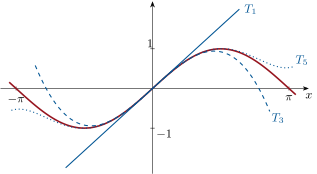
16.3 Applications

Example 16.15 (Limits)

\lim_{x \to 0} \frac{x - \sin x}{x^3}: \qquad x - \sin x = \frac{x^3}{6} + o(x^3) \sim \frac{x^3}{6}, \qquad\text{so the limit is } \frac16

— settling the question raised in Exercise 4.9. Likewise $\displaystyle\lim_{x\to0}\Bigl(\frac{\sin x}{x}\Bigr)^{1/x^2}$ : the logarithm is

\frac{1}{x^2}\ln\Bigl(1 - \frac{x^2}{6} + o(x^2)\Bigr) = \frac{1}{x^2}\Bigl(-\frac{x^2}{6} + o(x^2)\Bigr) \longrightarrow -\frac16, \qquad\text{limit } \eu^{-1/6}.

Remark 16.16 (Common pitfalls with expansions)

(i) Never add or subtract equivalents: from $\tan x \sim x$ and $\sin x \sim x$ one may not conclude $\tan x - \sin x \sim 0$ (meaningless) — the honest route is expansions:

\tan x - \sin x = \Bigl(x + \frac{x^3}{3}\Bigr) - \Bigl(x - \frac{x^3}{6}\Bigr) + o(x^3) = \frac{x^3}{2} + o(x^3) \sim \frac{x^3}{2} .

(ii) Expand past the massacre: in the same computation, order $1$ sees only $x - x = 0$ ; whenever leading terms cancel, raise the order until a nonzero coefficient survives, and only then convert back to an equivalent. (iii) Equivalents do not pass through exponentials: $n^2 + n \sim n^2$ , yet $\eu^{n^2+n} = \eu^{n}\,\eu^{n^2}$ is not equivalent to $\eu^{n^2}$ — exponentiate only expansions of the exponent whose error tends to $0$ , never equivalents of the exponent. (Logarithms are safer: if $u_n \sim v_n \to \ell \neq 1$ , $\ell > 0$ , then $\ln u_n \sim \ln v_n$ .) (iv) The $o(\cdot)$ calculus is one-directional: $o(x^2) + o(x^2) = o(x^2)$ , $5\,o(x^2) = o(x^2)$ , $x\cdot o(x^2) = o(x^3)$ — but an $o(x^2)$ is not a specific function, so never cancel two of them against each other: $o(x^2) - o(x^2)$ is $o(x^2)$ , not $0$ .

Proposition 16.17 (Local behavior)

Suppose $f(x) = f(a) + c\,(x - a)^p + o\bigl((x-a)^p\bigr)$ with $c \neq 0$ (first nonzero term after the constant; $p \geq 2$ at a critical point).

If $p$ is even: $f$ has a local minimum at $a$ if $c > 0$ , a local maximum if $c < 0$ .
If $p$ is odd: no extremum ( $f - f(a)$ changes sign); if moreover the expansion starts after a linear term $f'(a)(x - a)$ , the graph crosses its tangent: an inflection.

Proof. Near $a$ , $f(x) - f(a) = (x-a)^p\bigl(c + o(1)\bigr)$ has the sign of $c\,(x-a)^p$ : constant sign for $p$ even, changing for $p$ odd. ∎

Example 16.18 (Exponents must be expanded to $o(1)$ )

Find an equivalent of $u_n = \bigl(1 + \frac1n\bigr)^{n^2}$ . Expand the exponent until its error tends to $0$ :

n^2 \ln\Bigl(1 + \frac1n\Bigr) = n^2\Bigl(\frac1n - \frac{1}{2n^2} + O\Bigl(\frac{1}{n^3}\Bigr)\Bigr) = n - \frac12 + O\Bigl(\frac1n\Bigr),

so $u_n = \eu^{\,n - 1/2}\,\eu^{O(1/n)}$ with $\eu^{O(1/n)} \to 1$ :

u_n \;\sim\; \eu^{\,n - \frac12} .

Note what would have gone wrong with less care: stopping the exponent at $n^2\cdot\frac1n = n + O(1)$ leaves an $\eu^{O(1)}$ factor — bounded but not tending to $1$ — and no equivalent can be asserted. The rule of the pitfalls above, in positive form: an equivalent of $\eu^{a_n}$ requires the expansion of $a_n$ up to a term tending to zero, every coefficient before that being kept exactly.

Example 16.19 (Classifying a flat critical point)

Study $f(x) = \cos x + \frac{x^2}{2}$ near $0$ . Both $f'(0) = 0$ and $f''(0) = -\cos 0 + 1 = 0$ : the second-derivative test is mute. Expand instead:

f(x) = \Bigl(1 - \frac{x^2}{2} + \frac{x^4}{24} + o(x^4)\Bigr) + \frac{x^2}{2} = 1 + \frac{x^4}{24} + o(x^4) :

first nonzero term $c\,x^p$ with $p = 4$ even and $c = \frac{1}{24} > 0$ : a local minimum, of unusual flatness (the graph leaves its minimum value like $x^4$ , not $x^2$ ). The closing insight: the expansion sees in one line what iterated differentiation obscures — and Proposition 16.17 is the systematic dictionary from “first surviving term” to “local shape”.

Example 16.20 (Expansions at infinity)

Two computations where the variable runs to $+\infty$ and the substitution $h = \frac1x \to 0^+$ imports the whole toolbox. First,

x - x^2\ln\Bigl(1 + \frac1x\Bigr) = x - x^2\Bigl(\frac1x - \frac{1}{2x^2} + O\Bigl(\frac{1}{x^3}\Bigr)\Bigr) = \frac12 + O\Bigl(\frac1x\Bigr) \longrightarrow \frac12 .

Second, the arctangent at infinity: from $\arctan x + \arctan\frac1x = \frac\pi2$ for $x > 0$ (Proposition 4.12) and the expansion of $\arctan$ at $0$ (Exercise 16.3),

\arctan x = \frac\pi2 - \arctan\frac1x = \frac\pi2 - \frac1x + \frac{1}{3x^3} + o\Bigl(\frac{1}{x^3}\Bigr) :

the graph approaches its asymptote $y = \frac\pi2$ from below at speed $\frac1x$ . The closing insight: there is no separate theory of expansions at infinity — one reciprocal substitution reduces them to expansions at $0$ , provided every intermediate $O$ and $o$ is carried along honestly.

Example 16.21 (Asymptote by expansion)

As $x \to +\infty$ ,

\sqrt{x^2 + x} = x\sqrt{1 + \tfrac1x} = x\Bigl(1 + \frac{1}{2x} - \frac{1}{8x^2} + o\bigl(\tfrac{1}{x^2}\bigr)\Bigr) = x + \frac12 - \frac{1}{8x} + o\bigl(\tfrac 1x\bigr):

the line $y = x + \frac12$ is an asymptote, approached from below (the next term $-\frac{1}{8x}$ is negative).

Remark 16.22 (Where expansions work next)

Asymptotic expansions are the standing language of the rest of the book: in Chapter 17 they decide convergence (equivalents feed the comparison tests, and the study of $\sum \frac{1}{n^\alpha}$ is an expansion in disguise); in the Year 2 volume they become power series, where the Taylor polynomial acquires infinitely many terms and a radius of convergence; and every linearization in physics — the pendulum, first-order perturbation — is a Taylor–Young statement with the $o(\cdot)$ silently dropped. The one warning worth engraving: an expansion describes a function only near one point — see the flat function of the weekend problem, whose expansion at $0$ is identically zero without the function being so.

Remark 16.23 (Perspectives inside this volume)

Expansions are the working language of the remaining analysis and of the geometry to come. Chapter 17 converts them into convergence verdicts: an equivalent of the general term is an expansion truncated at its first term, and the finer tests (alternating with error control) consume the second term too. Chapter 24 reads local geometry from expansions of the two coordinate functions: whether a parametrized curve crosses, kisses, or cusps at a point is decided by which powers of $t$ survive in $x(t)$ and $y(t)$ — the plane version of Proposition 16.17. And Chapter 25 stops at order one on purpose: the tangent plane is a two-variable Taylor–Young statement, with the full second-order theory (Hessians, saddle points) deferred to the Year 2 volume. The common thread: every “local” question in this book is answered by writing down the first surviving term of an expansion.

16.4 Exercises

Exercise 16.1 ★

Give the expansions at $0$ : $\eu^{2x}$ to order $3$ ; $\;\ln(1 - x)$ to order $4$ ; $\;\sqrt{1 + x}$ to order $3$ ; $\;\dfrac{1}{1 + x^2}$ to order $6$ .

Solution

Solution of Exercise 16.1.

\eu^{2x} = 1 + 2x + 2x^2 + \frac{4x^3}{3} + o(x^3); \qquad \ln(1 - x) = -x - \frac{x^2}{2} - \frac{x^3}{3} - \frac{x^4}{4} + o(x^4);

\sqrt{1+x} = 1 + \frac x2 - \frac{x^2}{8} + \frac{x^3}{16} + o(x^3); \qquad \frac{1}{1 + x^2} = 1 - x^2 + x^4 - x^6 + o(x^6),

the last by substituting $-x^2$ into the geometric expansion.

Exercise 16.2 ★

Compute the limits:

\lim_{x\to 0} \frac{\eu^x - 1 - x}{x^2}, \qquad \lim_{x\to 0} \frac{\cos x - \sqrt{1 - x^2}}{x^4}, \qquad \lim_{x\to 0} \frac{\ln(1+x) - \sin x}{x^2}.

Solution

Solution of Exercise 16.2.

$\eu^x - 1 - x = \frac{x^2}{2} + o(x^2)$ : limit $\dfrac12$ .

$\cos x = 1 - \frac{x^2}{2} + \frac{x^4}{24} + o(x^4)$ and $\sqrt{1 - x^2} = 1 - \frac{x^2}{2} - \frac{x^4}{8} + o(x^4)$ : difference $\frac{x^4}{24} + \frac{x^4}{8} = \frac{x^4}{6} + o(x^4)$ : limit $\dfrac16$ .

$\ln(1+x) - \sin x = \bigl(x - \frac{x^2}{2}\bigr) - x + o(x^2) = -\frac{x^2}{2} + o(x^2)$ : limit $-\dfrac12$ .

Exercise 16.3 ★

Expand $\arctan x$ at $0$ to order $5$ by integrating the expansion of $\frac{1}{1 + x^2}$ , and $\arcsin x$ to order $5$ by integrating that of $(1 - x^2)^{-1/2}$ .

Solution

Solution of Exercise 16.3.

$\frac{1}{1+t^2} = 1 - t^2 + t^4 + o(t^5)$ ; integrating from $0$ to $x$ (Method 16.12 (5)):

\arctan x = x - \frac{x^3}{3} + \frac{x^5}{5} + o(x^5)\ \ (\text{even }o(x^6)\text{, by oddness}).

$(1 - t^2)^{-1/2} = 1 + \frac{t^2}{2} + \frac38 t^4 + o(t^5)$ (binomial expansion with $\alpha = -\frac12$ , $x = -t^2$ : $\binom{-1/2}{2} = \frac{(-\frac12)(-\frac32)}{2} = \frac38$ ); integrating:

\arcsin x = x + \frac{x^3}{6} + \frac{3x^5}{40} + o(x^5) .

Exercise 16.4 ★

Using Taylor–Lagrange for $\exp$ on $\intcc{0}{1}$ , prove that

\Bigl| \eu - \sum_{k=0}^{n} \frac{1}{k!} \Bigr| \leq \frac{3}{(n+1)!},

and determine an $n$ guaranteeing $6$ exact decimals of $\eu$ .

Solution

Solution of Exercise 16.4.

Taylor–Lagrange (Theorem 16.7) for $\exp$ at $a = 0$ , $x = 1$ : the $(n+1)$ -st derivative is $\eu^t \leq \eu < 3$ on $\intcc{0}{1}$ , so

\Bigl|\eu - \sum_{k=0}^{n} \frac{1}{k!}\Bigr| \leq \frac{3}{(n+1)!} .

For $6$ exact decimals, want $\frac{3}{(n+1)!} < 5\times 10^{-7}$ , i.e. $(n+1)! > 6\times 10^{6}$ : since $10! = 3\,628\,800$ and $11! = 39\,916\,800$ , $n + 1 = 11$ , i.e. $n = 10$ suffices.

Exercise 16.5 ★★

Expand to order $2$ in $\frac1n$ and deduce the limit and the speed of convergence:

\Bigl(1 + \frac 1n\Bigr)^{\!n} = \eu\Bigl(1 - \frac{1}{2n} + \frac{11}{24n^2} + o\Bigl(\frac{1}{n^2}\Bigr)\Bigr).

Solution

Solution of Exercise 16.5.

$n\ln\bigl(1 + \frac1n\bigr) = n\Bigl(\frac1n - \frac{1}{2n^2} + \frac{1}{3n^3} + o\bigl(\frac{1}{n^3}\bigr)\Bigr) = 1 - \frac{1}{2n} + \frac{1}{3n^2} + o\bigl(\frac{1}{n^2}\bigr)$ . Exponentiating, with $u = -\frac{1}{2n} + \frac{1}{3n^2}$ and $\eu^u = 1 + u + \frac{u^2}2 + o(u^2)$ :

\Bigl(1 + \frac1n\Bigr)^n = \eu\cdot \eu^{u} = \eu\Bigl(1 - \frac{1}{2n} + \frac{1}{3n^2} + \frac{1}{8n^2} + o\Bigl(\frac{1}{n^2}\Bigr)\Bigr) = \eu\Bigl(1 - \frac{1}{2n} + \frac{11}{24n^2} + o\Bigl(\frac{1}{n^2}\Bigr)\Bigr).

Limit $\eu$ ; the error is $\sim \dfrac{\eu}{2n}$ : slow (one digit per tenfold increase of $n$ ).

Exercise 16.6 ★★

Study the local behavior at $0$ of $f(x) = x^2 - x^4$ and of $g(x) = x^3 + x^5$ ; and find the position of the graph of $h(x) = \eu^x$ relative to its tangent at $a = 1$ , locally then globally.

Solution

Solution of Exercise 16.6.

$f(x) = x^2 - x^4 = x^2(1 + o(1))$ : first term $x^2$ , $p = 2$ even, coefficient $> 0$ : local minimum at $0$ (not global: $f(2) = -12$ ).

$g(x) = x^3 + x^5$ : first term $x^3$ , odd $p$ : no extremum; $g$ crosses its (horizontal) tangent: inflection at $0$ .

$h = \exp$ at $a = 1$ : $h(x) = \eu + \eu(x-1) + \frac{\eu}{2}(x-1)^2 + o((x-1)^2)$ ; the difference with the tangent is $\frac{\eu}{2}(x-1)^2 + o(\cdot) > 0$ locally. Globally: $\eu^x - \eu x \geq 0$ for all $x$ by convexity (Theorem 14.19 (3)): the graph lies above every tangent, with equality only at the contact point.

Exercise 16.7 ★★

Determine the asymptotes at $\pm\infty$ of $f(x) = \sqrt[3]{x^3 + x^2}$ and the position of the curve relative to them.

Solution

Solution of Exercise 16.7.

For $x \to +\infty$ :

f(x) = x\Bigl(1 + \frac1x\Bigr)^{1/3} = x\Bigl(1 + \frac{1}{3x} - \frac{1}{9x^2} + o\Bigl(\frac{1}{x^2}\Bigr)\Bigr) = x + \frac13 - \frac{1}{9x} + o\Bigl(\frac1x\Bigr):

asymptote $y = x + \frac13$ , curve below it near $+\infty$ . As $x \to -\infty$ , the same computation is valid (the cube root is defined for all reals, and $\frac1x \to 0$ ): same asymptote $y = x + \frac13$ , but now $-\frac{1}{9x} > 0$ : curve above the line.

Exercise 16.8 ★★

Find the equivalent, as $n \to \infty$ , of

u_n = \sqrt{n+1} - \sqrt n, \qquad v_n = \ln(n+1) - \ln n, \qquad w_n = \sin\frac{1}{n} - \tan\frac{1}{n},

each as a power of $n$ times a constant.

Solution

Solution of Exercise 16.8.

$u_n = \sqrt n\bigl(\sqrt{1 + \tfrac1n} - 1\bigr) = \sqrt n\bigl(\frac{1}{2n} + o(\frac1n)\bigr) \sim \dfrac{1}{2\sqrt n}$ .

$v_n = \ln\bigl(1 + \frac1n\bigr) \sim \dfrac 1n$ .

$w_n$ : with $h = \frac1n \to 0$ , $\sin h - \tan h = \bigl(h - \frac{h^3}{6}\bigr) - \bigl(h + \frac{h^3}{3}\bigr) + o(h^3) = -\frac{h^3}{2} + o(h^3)$ , so $w_n \sim -\dfrac{1}{2n^3}$ .

Exercise 16.9 ★★★

Let $f$ be $C^2$ on $\R$ . Prove that for every $x$ and $h > 0$ :

\abs{f'(x)} \leq \frac{\abs{f(x+h) - f(x-h)}}{2h} + \frac{h}{2}\sup_{\intcc{x-h}{x+h}}\abs{f''} ,

and deduce the Landau–Kolmogorov-type inequality: if $\abs f \leq M_0$ and $\abs{f''} \leq M_2$ on $\R$ , then $\abs{f'} \leq \sqrt{2 M_0 M_2}$ everywhere. (Optimize over $h$ .)

Solution

Solution of Exercise 16.9.

Taylor–Lagrange at order $1$ around $x$ , on both sides:

f(x + h) = f(x) + h f'(x) + R_+,\quad f(x - h) = f(x) - h f'(x) + R_-, \qquad \abs{R_\pm} \leq \frac{h^2}{2} \sup \abs{f''} .

Subtracting: $f(x+h) - f(x-h) = 2h f'(x) + (R_+ - R_-)$ , so

\abs{f'(x)} \leq \frac{\abs{f(x+h) - f(x-h)}}{2h} + \frac{h}{2}\sup_{\intcc{x-h}{x+h}}\abs{f''} .

With global bounds: $\abs{f'(x)} \leq \frac{M_0}{h} + \frac{M_2 h}{2}$ for every $h > 0$ . The right side is minimized at $h = \sqrt{2M_0/M_2}$ (derivative zero), with value $\sqrt{2M_0M_2}$ — hence $\abs{f'} \leq \sqrt{2M_0M_2}$ . (If $M_2 = 0$ , let $h \to \infty$ : $f' = 0$ , consistent.)

Exercise 16.10 ★★★

The sequence $u_0 \in \intoo{0}{\pi}$ , $u_{n+1} = \sin u_n$ decreases to $0$ (justify briefly). To find its speed, consider $v_n = \frac{1}{u_n^2}$ :

using the expansion of $\sin$ , prove $v_{n+1} - v_n \to \frac13$ ;
with Cesàro (Exercise 11.10), deduce $\frac{v_n}{n} \to \frac13$ , then the equivalent $u_n \sim \sqrt{\dfrac{3}{n}}$ .

Solution

Solution of Exercise 16.10.

On $\intoo{0}{\pi}$ : $0 < \sin u < u$ , so $(u_n)$ is strictly decreasing, positive, hence convergent; the limit is a fixed point of $\sin$ in $\intcc{0}{\pi}$ , and $\sin \ell = \ell$ forces $\ell = 0$ (since $\sin x < x$ for $x > 0$ ).

Using $\sin u = u - \frac{u^3}{6} + o(u^3)$ as $u \to 0$ :

$v_{n+1} - v_n = \frac{1}{\sin^2 u_n} - \frac{1}{u_n^2} = \frac{1}{u_n^2}\Bigl(\Bigl(1 - \frac{u_n^2}{6} + o(u_n^2)\Bigr)^{\!-2} - 1\Bigr) = \frac{1}{u_n^2}\Bigl(\frac{u_n^2}{3} + o(u_n^2)\Bigr) \longrightarrow \frac13 .$
By Exercise 11.10 (3) (Cesàro for differences), $\frac{v_n}{n} \to \frac13$ , i.e. $v_n \sim \frac n3$ , i.e. $u_n^2 \sim \frac 3n$ : since $u_n > 0$ ,

$u_n \sim \sqrt{\frac{3}{n}} .$

Exercise 16.11 ★★

(Differences of infinities) Compute

\lim_{x \to 0} \Bigl(\frac{1}{x^2} - \frac{1}{\sin^2 x}\Bigr) \qquad\text{and}\qquad \lim_{x \to 0^+} \Bigl(\frac 1x - \frac{1}{\ln(1 + x)}\Bigr)

by reducing to a common denominator and expanding numerator and denominator separately.

Solution

Solution of Exercise 16.11.

Common denominators. First limit:

\frac{1}{x^2} - \frac{1}{\sin^2 x} = \frac{\sin^2 x - x^2}{x^2\sin^2 x}, \qquad \sin^2 x = \Bigl(x - \frac{x^3}{6} + o(x^4)\Bigr)^{\!2} = x^2 - \frac{x^4}{3} + o(x^5) ,

so the numerator is $-\frac{x^4}{3} + o(x^4)$ while the denominator is $\sim x^4$ : the limit is $-\dfrac13$ .

Second: $\dfrac1x - \dfrac{1}{\ln(1+x)} = \dfrac{\ln(1+x) - x}{x\ln(1+x)}$ ; the numerator is $-\frac{x^2}{2} + o(x^2)$ , the denominator $x\bigl(x + o(x)\bigr) \sim x^2$ : the limit is $-\dfrac12$ .

Exercise 16.12 ★★★

(Asymptotics of implicit roots) Show that for every $k \in \N^*$ the equation $\tan x = x$ has exactly one solution $x_k$ in $\intoo{k\pi - \frac\pi2}{k\pi + \frac\pi2}$ , that $x_k = k\pi + \frac\pi2 - \varepsilon_k$ with $\varepsilon_k = \arctan\frac{1}{x_k}$ , and deduce the expansion

x_k = k\pi + \frac\pi2 - \frac{1}{k\pi} + o\Bigl(\frac 1k\Bigr) \qquad (k \to \infty).

Solution

Solution of Exercise 16.12.

On $I_k = \intoo{k\pi - \frac\pi2}{k\pi + \frac\pi2}$ , the function $g(x) = \tan x - x$ has derivative $\tan^2 x \geq 0$ , vanishing only at the single point $k\pi$ : $g$ is strictly increasing on $I_k$ (Corollary 14.12 (2)), with limits $-\infty$ and $+\infty$ at the ends: exactly one zero $x_k$ . For $k \geq 1$ , $g(k\pi) = -k\pi < 0$ , so $x_k \in \intoo{k\pi}{k\pi + \frac\pi2}$ : write $x_k = k\pi + \frac\pi2 - \varepsilon_k$ with $\varepsilon_k \in \intoo{0}{\frac\pi2}$ . Then

x_k = \tan x_k = \tan\Bigl(\frac\pi2 - \varepsilon_k\Bigr) = \frac{1}{\tan\varepsilon_k} \quad\Longrightarrow\quad \varepsilon_k = \arctan\frac{1}{x_k} ,

using $\tan\varepsilon_k = \frac{1}{x_k}$ and $\varepsilon_k \in \intoo{0}{\frac\pi2}$ . Since $x_k \geq k\pi \to \infty$ : $\varepsilon_k \to 0$ , and

\varepsilon_k = \arctan\frac{1}{x_k} = \frac{1}{x_k} + O\Bigl(\frac{1}{x_k^3}\Bigr) = \frac{1}{k\pi + O(1)} + O\Bigl(\frac{1}{k^3}\Bigr) = \frac{1}{k\pi} + O\Bigl(\frac{1}{k^2}\Bigr) ,

whence $x_k = k\pi + \frac\pi2 - \frac{1}{k\pi} + o\bigl(\frac1k\bigr)$ .

16.5 Problem: Alternating sums, certified digits, and the irrationality of $\cos 1$

Problem 16.1

Weekend problem — the alternating estimate $\abs{S - S_n} \leq a_{n+1}$ : $\ln 2$ and $\pi$ with proven decimals, Machin’s formula, and $\cos 1 \notin \Q$

An alternating sum with decreasing terms is the friendliest object in numerical analysis: its error is bounded by the first omitted term, with known sign. This problem proves that principle with the adjacent-sequences theorem, then spends it three ways: certified decimals for $\ln 2$ (three competing routes) and for $\pi$ (Leibniz, then Machin’s 1706 formula, still the idea behind record computations for centuries), the irrationality of $\cos 1$ , $\sin 1$ and $\cosh 1$ , and, as a counterweight, the Taylor–Lagrange equality and the flat function whose Taylor expansion lies. Throughout, “series” language is informal: every sum here is a sequence of partial sums, as in Example 11.12; the theory proper opens in Chapter 17.

Part I — The alternating estimate. Let $(a_k)_{k \geq 0}$ decrease to $0$ and $S_n = \sum_{k=0}^{n} (-1)^k a_k$ .

Show that $(S_{2n+1})$ is nondecreasing, $(S_{2n})$ nonincreasing, and that they are adjacent (Theorem 11.11): both converge to a common $S$ with, for every $n$ ,

$S_{2n+1} \leq S \leq S_{2n}, \qquad \abs{S - S_n} \leq a_{n+1} ,$

the error having the sign of the first omitted term. Show moreover that if the decrease is strict, all these inequalities are strict.
First dividend: for $x = 1$ in the exponential series, compare with Theorem 16.7 at $a = 0$ : show that $T_n = \sum_{k=0}^{n} \frac{(-1)^k}{k!}$ converges to $\eu^{-1}$ with $\abs{\eu^{-1} - T_n} < \frac{1}{(n+1)!}$ .
(Leibniz, 1674) From the exact finite identity

$\frac{1}{1 + t^2} = \sum_{k=0}^{n} (-1)^k t^{2k} + \frac{(-1)^{n+1} t^{2n+2}}{1 + t^2} ,$

integrated over $\intcc{0}{1}$ , prove

$\frac\pi4 = \sum_{k=0}^{n} \frac{(-1)^k}{2k+1} + \rho_n, \qquad \abs{\rho_n} \leq \frac{1}{2n+3} .$
Slowness: how many terms of Leibniz guarantee six exact decimals of $\pi$ ? (About two million.) Evaluate $4 S_4 = 4\bigl(1 - \frac13 + \frac15 - \frac17 + \frac19\bigr)$ and its distance to $\pi$ , to feel the pain.

Part II — $\ln 2$ three ways.

(Way 1: alternating harmonic) From $\frac{1}{1+t} = \sum_{k=0}^{n-1}(-1)^k t^k + \frac{(-1)^n t^n}{1+t}$ integrated over $\intcc{0}{1}$ :

$\ln 2 = \sum_{k=1}^{n} \frac{(-1)^{k-1}}{k} + (-1)^n R_n, \qquad \frac{1}{2(n+1)} \leq R_n \leq \frac{1}{n+1} :$

the error is of exact order $\frac 1n$ — a million terms for six decimals.
(Way 2: the fast series) Integrate $\frac{1}{1 - t^2} = \sum_{k=0}^{n} t^{2k} + \frac{t^{2n+2}}{1-t^2}$ from $0$ to $x \in \intoo{0}{1}$ and evaluate at $x = \frac13$ (note $\frac{1 + 1/3}{1 - 1/3} = 2$ ):

$\ln 2 = 2\sum_{k=0}^{n} \frac{(1/3)^{2k+1}}{2k+1} + \tilde\rho_n, \qquad 0 < \tilde\rho_n \leq \frac{9}{4}\cdot \frac{(1/3)^{2n+3}}{2n+3} :$

geometric convergence, roughly one digit per term.
(Way 3: Riemann sums and a hidden identity) Prove by induction the identity

$\sum_{k=1}^{2n} \frac{(-1)^{k-1}}{k} = H_{2n} - H_n = \sum_{k=1}^{n} \frac{1}{n + k} ,$

and recover $\ln 2$ as the Riemann-sum limit of Example 15.21: Ways 1 and 3 are secretly the same number seen twice.
Shootout at six terms: compare $\sum_{k=1}^{6} \frac{(-1)^{k-1}}{k} = 0.6167$ with Way 2 at $n = 5$ , which already gives $\ln 2 = 0.693147$ with error $\leq 1.1\cdot10^{-7}$ . Explain the structural reason (evaluation point deep inside the interval of convergence versus on its boundary).
How many terms of Way 2 certify ten decimals of $\ln 2$ ? Show $n = 10$ suffices.

Part III — Machin’s formula.

Compute $(5 + \iu)^4$ and verify the complex identity

$(5 + \iu)^4 = 2\,(1 + \iu)\,(239 + \iu) .$

Taking arguments (Chapter 3 conventions), deduce Machin’s formula

$\frac\pi4 = 4\arctan\frac15 - \arctan\frac{1}{239} .$

(Check that no argument leaves $\intoo{-\frac\pi2}{\frac\pi2}$ .)
As in question 3, establish for $0 < x < 1$ :

$\arctan x = \sum_{k=0}^{n} \frac{(-1)^k x^{2k+1}}{2k+1} + r_n(x), \qquad \abs{r_n(x)} \leq \frac{x^{2n+3}}{2n+3} .$
Certify $\pi$ to seven decimals with six terms: bound the total error of

$\pi \approx 16\sum_{k=0}^{4} \frac{(-1)^k (1/5)^{2k+1}}{2k+1} - 4\Bigl(\frac{1}{239} - \frac{1}{3\cdot239^3}\Bigr)$

by $16\,\frac{(1/5)^{11}}{11} + 4\,\frac{(1/239)^5}{5} < 5\cdot10^{-8}$ , and give the resulting value $3.1415926\dots$
Compare the three routes to $\pi$ now available — Leibniz (question 4), the Dalzell integrals of Problem 15.1 (error $4^{1-5m}$ ), Machin (error $\approx 16\cdot 5^{-(2n+3)}$ ) — in digits per term, and explain why shrinking the evaluation point beats everything.

Part IV — The integer trap, alternating edition.

Suppose $\cos 1 = \frac pq$ . Multiply the strict alternating bracketing of $\sum_{k} \frac{(-1)^k}{(2k)!}$ (question 1) by $(2n)!$ with $2n \geq q$ , and derive a contradiction: $\cos 1$ is irrational.
Adapt to $\sin 1 = \sum_k \frac{(-1)^k}{(2k+1)!}$ (multiply by $(2n+1)!$ ): $\sin 1 \notin \Q$ . Both irrational, yet $\cos^2 1 + \sin^2 1 = 1$ : irrationality is not stable under algebra.
The non-alternating cousin: $\cosh 1 = \sum_k \frac{1}{(2k)!}$ (in the partial-sum sense, with the two-sided tail bound $0 < \cosh 1 - \sum_{k \leq n} \frac{1}{(2k)!} < \frac{2}{(2n+2)!}$ , to be proved). Conclude $\cosh 1 \notin \Q$ by the same trap.
Push to $\cos\frac 1m$ for every integer $m \geq 1$ : multiply by $m^{2n}(2n)!$ and conclude $\cos\frac1m \notin \Q$ . Where does the same attempt break for $\cos\frac ab$ with $b > 1$ general? (Identify the denominator that no longer clears.)

Part V — Sharper and darker: the equality form, and a function that fools Taylor.

(Taylor–Lagrange, equality form) Let $f$ be $n + 1$ times differentiable between $a$ and $x$ . Define $g(t) = f(x) - \sum_{k=0}^{n} \frac{f^{(k)}(t)}{k!}(x - t)^k - A\,\frac{(x-t)^{n+1}}{(n+1)!}$ with the constant $A$ chosen so that $g(a) = 0$ . Compute $g'$ (the sum telescopes), apply Rolle on $\intcc{a}{x}$ , and conclude that there exists $c$ strictly between $a$ and $x$ with

$f(x) = \sum_{k=0}^{n} \frac{f^{(k)}(a)}{k!}(x-a)^k + \frac{f^{(n+1)}(c)}{(n+1)!}\,(x-a)^{n+1} .$
Dividend of the equality: for $x > 0$ show

$\eu^x > 1 + x + \frac{x^2}{2!} + \dots + \frac{x^n}{n!}$

(strictly, for every $n$ ), and locate where the inequality reverses for $x < 0$ according to the parity of $n$ .
Benchmark the remainders on $\sin(0.5)$ at order $3$ : Young gives only $o(x^3)$ (no number); Lagrange gives $\abs{\sin 0.5 - (0.5 - \frac{0.5^3}{6})} \leq \frac{0.5^5}{120} = 2.61\cdot10^{-4}$ ; the alternating estimate gives the same bound plus the sign information $\sin 0.5 > 0.5 - \frac{0.5^3}{6}$ . Compare with the true error $2.59\cdot10^{-4}$ : the bound is nearly attained. Which tool would you reach for, and when?
(The flat function) Let $f(x) = \eu^{-1/x^2}$ for $x \neq 0$ , $f(0) = 0$ . Show $f$ is continuous at $0$ , that $f'(0) = 0$ , and more generally — by proving that every derivative has the form $f^{(k)}(x) = P_k\bigl(\frac1x\bigr)\eu^{-1/x^2}$ for a polynomial $P_k$ (induction) — that $f^{(k)}(0) = 0$ for all $k$ (growth comparison Proposition 4.6). Conclude: all Taylor polynomials of $f$ at $0$ vanish, yet $f(x) > 0$ for $x \neq 0$ : Taylor–Young holds at every order, and says nothing about $f$ away from $0$ . Expansions describe germs, not functions.

Part VI — Synthesis.

Run the trap once more, on $\eu^{-1} = \sum_k \frac{(-1)^k}{k!}$ : multiply the strict alternating bracketing by $n!$ and conclude $\eu^{-1} \notin \Q$ , hence $\eu \notin \Q$ — the third proof of this fact in the volume. List the three (adjacent sequences, Exercise 11.9; integrals, Problem 15.1; alternating sums, here) and what each needed.
The fine print: monotonicity is not decorative. Let $b_k = \frac1k$ for odd $k$ and $b_k = \frac{1}{k^2}$ for even $k$ : the $b_k$ are positive and tend to $0$ , yet the partial sums of $\sum (-1)^k b_k$ diverge to $-\infty$ . Prove it (split the partial sum into the even part, bounded via Example 11.22, and the odd part, which dominates half the harmonic series, Exercise 11.5), and say exactly which step of question 1 used monotonicity.
Verify Euler’s simpler identity $\arctan\frac12 + \arctan\frac13 = \frac\pi4$ via $(2 + \iu)(3 + \iu) = 5(1 + \iu)$ , estimate the terms needed for six decimals of $\pi$ by this route ( $n = 10$ suffices), and place it between Leibniz and Machin in the ranking of question 13.
Synthesis, one sentence each: (i) state the alternating estimate and its two outputs (bound and sign); (ii) why exact finite identities with explicit remainders beat limit statements for certified numerics; (iii) inventory of the problem ( $\pi$ to $10^{-7}$ by hand, $\ln 2$ to ten decimals, four irrationality proofs, one equality theorem, one warning example); (iv) which of these threads Chapter 17 will pick up (the alternating series test, absolute versus conditional convergence, and the rearrangement drama of its weekend problem).

Solution

Solution of Problem 16.1.

1. $S_{2n+1} - S_{2n-1} = a_{2n} - a_{2n+1} \geq 0$ and $S_{2n+2} - S_{2n} = a_{2n+2} - a_{2n+1} \leq 0$ , while $S_{2n} - S_{2n+1} = a_{2n+1} \to 0$ : the sequences $(S_{2n+1})$ , $(S_{2n})$ are adjacent, converging to a common $S$ (Theorem 11.11) with $S_{2n+1} \leq S \leq S_{2n}$ . For even $n$ : $S_{n+1} \leq S \leq S_n$ gives $-a_{n+1} \leq S - S_n \leq 0$ ; for odd $n$ : $0 \leq S - S_n \leq a_{n+1}$ . In both cases $\abs{S - S_n} \leq a_{n+1}$ and $S - S_n$ has the sign of $(-1)^{n+1}$ , the first omitted term. Strict decrease makes every displayed inequality strict, in particular $0 < \abs{S - S_n} < a_{n+1}$ .

2. $a_k = \frac{1}{k!}$ decreases strictly to $0$ : question 1 applies. Taylor–Lagrange (Theorem 16.7) for $\exp$ between $-1$ and $0$ : $\abs{\eu^{-1} - T_n} \leq \frac{1}{(n+1)!}$ (the derivative $\eu^t$ is $\leq 1$ there), so $T_n \to \eu^{-1}$ , and the limit $S$ of question 1 is $\eu^{-1}$ , with the strict bounds $0 < \abs{\eu^{-1} - T_n} < \frac{1}{(n+1)!}$ .

3. Integrating the identity over $\intcc{0}{1}$ : the left side is $\arctan 1 = \frac\pi4$ (fundamental theorem), the $k$ -th term gives $\frac{(-1)^k}{2k+1}$ , and

\rho_n = (-1)^{n+1}\int_0^1 \frac{t^{2n+2}}{1+t^2}\dd t, \qquad \abs{\rho_n} \leq \int_0^1 t^{2n+2}\dd t = \frac{1}{2n+3} .

4. The error on $\pi$ is $4\abs{\rho_n} \leq \frac{4}{2n+3}$ : below $10^{-6}$ requires $2n + 3 > 4\cdot10^6$ , about two million terms. Meanwhile $4S_4 = 4\bigl(1 - \frac13 + \frac15 - \frac17 + \frac19\bigr) = 4 \times 0.834921 = 3.339683$ , almost $0.2$ away from $\pi$ : five terms, not even one digit.

5. Integrating over $\intcc{0}{1}$ : $\ln 2 = \sum_{k=1}^{n} \frac{(-1)^{k-1}}{k} + (-1)^n R_n$ with $R_n = \int_0^1 \frac{t^n}{1+t}\dd t$ ; from $\frac12 \leq \frac{1}{1+t} \leq 1$ : $\frac{1}{2(n+1)} \leq R_n \leq \frac{1}{n+1}$ . The error is trapped between two multiples of $\frac1n$ : six decimals cost about a million terms.

6. Integrating from $0$ to $x$ : $\frac12\ln\frac{1 + x}{1 - x} = \sum_{k=0}^{n} \frac{x^{2k+1}}{2k+1} + \int_0^x \frac{t^{2n+2}}{1-t^2}\dd t$ . At $x = \frac13$ : $\frac{1 + 1/3}{1 - 1/3} = 2$ , and on $\intcc{0}{\frac13}$ , $\frac{1}{1 - t^2} \leq \frac98$ :

\ln 2 = 2\sum_{k=0}^{n} \frac{(1/3)^{2k+1}}{2k+1} + \tilde\rho_n, \qquad 0 < \tilde\rho_n \leq \frac{9}{4}\cdot \frac{(1/3)^{2n+3}}{2n+3} :

each extra term divides the error by about $9$ .

7. Induction: for $n = 1$ : $1 - \frac12 = \frac12 = H_2 - H_1$ . Step:

H_{2n+2} - H_{n+1} = (H_{2n} - H_n) + \frac{1}{2n+1} + \frac{1}{2n+2} - \frac{1}{n+1} = (H_{2n} - H_n) + \frac{1}{2n+1} - \frac{1}{2n+2},

which is exactly the increment of the alternating sum. And $H_{2n} - H_n = \sum_{k=1}^{n}\frac{1}{n+k}$ is the Riemann sum of Example 15.21, converging to $\ln 2$ : the even partial sums of Way 1 are the Riemann sums of Way 3.

8. $\sum_{k=1}^{6}\frac{(-1)^{k-1}}{k} = 0.61667$ , error $0.0765$ ; Way 2 at $n = 5$ gives $0.6931471$ with error $\leq \frac94\cdot\frac{(1/3)^{13}}{13} = 1.1\cdot10^{-7}$ . The reason: Way 1 evaluates the logarithm series at the boundary point $x = 1$ , where the terms decay like $\frac1k$ ; Way 2 evaluates at $x = \frac13$ , deep inside, where each term carries a fresh factor $\frac19$ .

9. Ten decimals: want $\tilde\rho_n \leq 5\cdot10^{-11}$ . At $n = 10$ : $\frac94 \cdot \frac{(1/3)^{23}}{23} = \frac94\cdot\frac{1.06\cdot10^{-11}}{23} \approx 1.0\cdot10^{-12} < 5\cdot10^{-11}$ : eleven terms suffice.

10. $(5+\iu)^2 = 24 + 10\iu$ , then $(5+\iu)^4 = (24 + 10\iu)^2 = 476 + 480\iu$ ; and $2(1+\iu)(239+\iu) = 2(238 + 240\iu) = 476 + 480\iu$ : equal. Arguments: $\arg(5 + \iu) = \arctan\frac15$ , so the left side has argument $4\arctan\frac15 \approx 0.79 \in \intoo{0}{\pi}$ ; the right side has argument $\frac\pi4 + \arctan\frac{1}{239} \in \intoo{0}{\pi}$ . Two equal complex numbers with arguments in the same interval of length $< 2\pi$ :

4\arctan\frac15 = \frac\pi4 + \arctan\frac{1}{239} ,

which is Machin’s formula.

11. Integrate $\frac{1}{1+t^2} = \sum_{k=0}^n (-1)^k t^{2k} + \frac{(-1)^{n+1}t^{2n+2}}{1+t^2}$ from $0$ to $x$ :

\arctan x = \sum_{k=0}^{n}\frac{(-1)^k x^{2k+1}}{2k+1} + r_n(x), \qquad \abs{r_n(x)} \leq \int_0^x t^{2n+2}\dd t = \frac{x^{2n+3}}{2n+3} .

12. Errors: $16\,\frac{(1/5)^{11}}{11} = 3.0\cdot 10^{-8}$ and $4\,\frac{(1/239)^5}{5} \approx 1\cdot10^{-12}$ : total $< 5\cdot10^{-8}$ . The displayed sum evaluates to $3.14159268\dots$ , hence $\pi = 3.1415926\dots$ certified to $5\cdot10^{-8}$ : seven decimals from six terms (five at $\frac15$ , two at $\frac1{239}$ counting generously).

13. Leibniz: error $\sim \frac1n$ , so each new digit multiplies the workload by ten. Dalzell (Problem 15.1, question 22): error $4^{1-5m}$ , about three digits per step, each step a heavier polynomial. Machin: error ratio $\frac{1}{25}$ per term, about $1.4$ digits per term, each term one division. The moral: the remainder of a geometric-type expansion scales like $x^{2n}$ , so making $x$ small buys digits at a fixed cost per term — Machin’s complex identity is precisely a machine for shrinking $x$ .

14. $a_k = \frac{1}{(2k)!}$ decreases strictly to $0$ ; by question 1 and Proposition 16.11 (Lagrange bound as in question 2), $\sum_{k \leq n}\frac{(-1)^k}{(2k)!} \to \cos 1$ with the strict bracket $0 < \bigl|\cos 1 - S'_n\bigr| < \frac{1}{(2n+2)!}$ . Suppose $\cos 1 = \frac pq$ and take $2n \geq q$ : then $(2n)!\,S'_n = \sum_{k\leq n} (-1)^k \frac{(2n)!}{(2k)!} \in \Z$ and $(2n)!\,\frac pq \in \Z$ , while

0 < \Bigl|(2n)!\cos 1 - (2n)!S'_n\Bigr| < \frac{(2n)!}{(2n+2)!} = \frac{1}{(2n+1)(2n+2)} < 1 :

a nonzero integer of absolute value $< 1$ . Contradiction: $\cos 1 \notin \Q$ .

15. Identically with $a_k = \frac{1}{(2k+1)!}$ , multiplying by $(2n+1)!$ with $2n + 1 \geq q$ : $\sin 1 \notin \Q$ . Yet $\cos^2 1 + \sin^2 1 = 1 \in \Q$ : products and sums of irrationals may be rational — irrationality passes through no algebraic operation for free.

16. Tail bound: for $m > n$ ,

\sum_{k=n+1}^{m} \frac{1}{(2k)!} \leq \frac{1}{(2n+2)!}\Bigl(1 + \frac12 + \frac14 + \dots\Bigr) \leq \frac{2}{(2n+2)!} ,

since each successive ratio is $\frac{1}{(2k+1)(2k+2)} \leq \frac12$ ; the tail is positive (its first term is). So $0 < \cosh 1 - \sum_{k\leq n}\frac{1}{(2k)!} < \frac{2}{(2n+2)!}$ , and multiplying by $(2n)!$ with $2n \geq q$ traps a nonzero integer in $\intoo{0}{1}$ again: $\cosh 1 \notin \Q$ .

17. $\cos\frac1m = \sum_k \frac{(-1)^k}{m^{2k}(2k)!}$ : the terms decrease strictly to zero, and $m^{2n}(2n)!\cdot\frac{1}{m^{2k}(2k)!} = m^{2(n-k)}\frac{(2n)!}{(2k)!} \in \Z$ for $k \leq n$ . If $\cos\frac1m = \frac pq$ , multiply the strict bracket by $q\,m^{2n}(2n)!$ : the error is bounded by $\frac{q}{m^2(2n+1)(2n+2)} < 1$ for large $n$ : contradiction. For $\frac ab$ with $a \geq 2$ : clearing denominators multiplies the tail by $b^{2n}(2n)!$ , but the first omitted term is $\frac{a^{2n+2}}{b^{2n+2}(2n+2)!}$ , and the product $\frac{a^{2n+2}}{b^2(2n+1)(2n+2)}$ explodes: the numerator $a^{2n+2}$ no longer clears, and the trap jams. (The result is still true — via Niven-style machinery, not this one.)

18. At $t = x$ every term of $g$ vanishes except $f(x) - f(x) = 0$ : $g(x) = 0$ ; $A$ is chosen so $g(a) = 0$ . Differentiating, the sum telescopes:

g'(t) = -\frac{f^{(n+1)}(t)}{n!}(x - t)^n + A\,\frac{(x-t)^n}{n!} = \frac{(x-t)^n}{n!}\bigl(A - f^{(n+1)}(t)\bigr) .

Rolle on the segment from $a$ to $x$ gives $c$ strictly between with $g'(c) = 0$ ; since $(x - c)^n \neq 0$ : $A = f^{(n+1)}(c)$ . Unfolding $g(a) = 0$ yields the Taylor equality with remainder $\frac{f^{(n+1)}(c)}{(n+1)!}(x-a)^{n+1}$ .

19. For $x > 0$ , the remainder is $\frac{\eu^{c}} {(n+1)!}x^{n+1} > 0$ : the exponential exceeds each of its Taylor polynomials, strictly, at every order. For $x < 0$ the sign of the remainder is that of $x^{n+1}$ : $\eu^x$ is above the polynomial for $n$ odd, below it for $n$ even — alternating sides, as the graphs of $1 + x$ and $1 + x + \frac{x^2}{2}$ against $\eu^x$ already show.

20. True error: $\sin 0.5 - 0.4791667 = 2.59\cdot10^{-4}$ , against the bound $\frac{0.5^5}{120} = 2.60\cdot10^{-4}$ : nearly attained (the next term dominates the tail). Young: for limits and local analysis, where no constant is needed. Lagrange: for certified decimals. Alternating: when applicable, same bound plus the direction of the error — the best of the three, but the rarest.

21. Continuity at $0$ : with $u = \frac{1}{x^2} \to +\infty$ , $f(x) = \eu^{-u} \to 0 = f(0)$ . Derivative at $0$ : $\bigl|\frac{f(h)}{h}\bigr| = \sqrt u\,\eu^{-u} \to 0$ (Proposition 4.6): $f'(0) = 0$ . For $x \neq 0$ , $f'(x) = \frac{2}{x^3}\eu^{-1/x^2}$ : the form $P_1\bigl(\frac1x\bigr)\eu^{-1/x^2}$ with $P_1(X) = 2X^3$ ; inductively, differentiating $P_k(\frac1x)\eu^{-1/x^2}$ gives $P_{k+1}(X) = 2X^3 P_k(X) - X^2 P_k'(X)$ , a polynomial. Then

\frac{f^{(k)}(h) - 0}{h} = v\,P_k(v)\,\eu^{-v^2} \Big|_{v = 1/h} \longrightarrow 0

(polynomial against $\eu^{-v^2}$ , growth comparison at $\pm\infty$ ): by induction $f^{(k)}(0) = 0$ for all $k$ . All Taylor polynomials of $f$ at $0$ vanish, yet $f > 0$ off $0$ : Taylor–Young is exact at every order and blind beyond the germ. An expansion is local information only.

22. By question 2, $0 < \abs{\eu^{-1} - T_n} < \frac{1}{(n+1)!}$ , strictly. If $\eu^{-1} = \frac pq$ , take $n \geq q$ and multiply by $n!$ : $n!\,T_n \in \Z$ and $n!\frac pq \in \Z$ , so a nonzero integer has absolute value $< \frac{n!}{(n+1)!} = \frac{1}{n+1} < 1$ : contradiction. Hence $\eu^{-1} \notin \Q$ , and $\eu = \frac{1}{\eu^{-1}}$ is irrational too. The three proofs: adjacent sequences squeezing $q!\,\eu$ (Exercise 11.9); the integral recurrence $A_n = \eu - nA_{n-1}$ (Problem 15.1); the alternating bracket (here). One trap, three certificates of smallness.

23. Group the partial sums in pairs: $\sum_{k=1}^{2n} (-1)^k b_k = E_n - O_n$ with $E_n = \sum_{j=1}^{n} \frac{1}{4j^2}$ , bounded (by the telescoping bound of Example 11.22, $E_n \leq \frac12$ ), and $O_n = \sum_{j=1}^{n}\frac{1}{2j-1} \geq \frac12 H_n \to +\infty$ (Exercise 11.5): the partial sums tend to $-\infty$ . Monotonicity was used in question 1 exactly where $S_{2n+1} - S_{2n-1} = a_{2n} - a_{2n+1}$ needed a sign: without decrease, the even and odd subsequences need not be monotone, and adjacency collapses.

24. $(2+\iu)(3+\iu) = 5 + 5\iu = 5(1+\iu)$ ; taking arguments (all in $\intoo{0}{\frac\pi2}$ ): $\arctan\frac12 + \arctan\frac13 = \frac\pi4$ . Series cost for six decimals: error $\leq 4\bigl(\frac{(1/2)^{2n+3}}{2n+3} + \frac{(1/3)^{2n+3}}{2n+3}\bigr)$ , which at $n = 10$ is $\approx 2\cdot10^{-8} < 5\cdot10^{-7}$ : eleven terms. Ranking: better than Leibniz by an exponential margin, behind Machin (whose dominant point $\frac15$ is smaller than $\frac12$ ): roughly $0.6$ digits per term against Machin’s $1.4$ .

25. (i) For decreasing $a_k \to 0$ , the alternating partial sums converge with $\abs{S - S_n} \leq a_{n+1}$ and the error carries the sign of the first omitted term. (ii) A finite identity with explicit remainder can be evaluated and bounded at a chosen point, while a limit statement only promises eventual closeness — certification needs the former. (iii) Extracted: $\pi$ to $5\cdot10^{-8}$ by Machin, $\ln 2$ to ten decimals by the $\frac13$ -series, irrationality of $\cos 1$ , $\sin 1$ , $\cosh 1$ , $\cos\frac1m$ and $\eu^{-1}$ , the Taylor–Lagrange equality, and the flat-function warning. (iv) Chapter 17 upgrades question 1 into the alternating series test, separates absolute from conditional convergence, and its weekend problem stages the rearrangement drama for which the alternating harmonic series of Way 1 is the star witness.

16.1 Comparison notation

16.2 The three Taylor formulas

16.3 Applications

16.4 Exercises

16.5 Problem: Alternating sums, certified digits, and the irrationality of cos⁡1\cos 1cos1

16.5 Problem: Alternating sums, certified digits, and the irrationality of $\cos 1$