Markets I: The Ecosystem and Exchange-Traded Markets · Markets

25Volatility as a Traded Quantity: First Contact

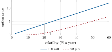
The three-month 100 call is offered at 4.06. Nobody on an options desk says so. They say the call is “twenty vol”; that the 90 put is “twenty-four”; that the stock’s “skew is six points”; that “the forward is 100.20, so the market has an 80-cent dividend in”. Prices in dollars change every time the share ticks; these numbers do not, and so they are what the desk quotes, compares, remembers and trades. This chapter learns the language. It needs one formula from outside (the Black–Scholes price, derived in One Quant Book 5 and used here as a black box that turns a volatility into a price) and one identity that needs no model at all.

25.1 Put–call parity, with dividends and borrow

Proposition 25.1 (Put–call parity)

For European options with the same strike $K$ and expiry $T$ on the same underlying,

C - P \;=\; \mathrm{e}^{-rT}\,(F - K),

where $F$ is the forward price of the underlying for $T$ : the put–call parity. For a share, $F\,\mathrm{e}^{-rT} = S - D$ , with $D$ the present value of the dividends paid before $T$ , to which a short seller adds the borrow fee.

Proof. Long a call and short a put at $K$ is an obligation to buy at $K$ at $T$ : a forward contract struck at $K$ , worth $\mathrm{e}^{-rT}(F-K)$ today. ∎

Parity holds whatever the volatility, the distribution or the model. It is enforced by two trades that a market maker can do mechanically: the conversion (buy the share, buy the put, sell the call) and the reversal (the opposite, which needs a stock borrow). Read backwards, it is a measuring instrument:

Method 25.2 (Reading the forward off the chain)

At each strike compute $F_K = K + \mathrm{e}^{rT}(C_K - P_K)$ from mid-prices. The values should agree to within the quotes’ width; average the ones near the money.
The implied carry is $D^{\text{imp}} = S - \mathrm{e}^{-rT}F$ : expected dividends plus the borrow fee that the marginal arbitrageur pays.
If $D^{\text{imp}}$ exceeds any plausible dividend, the share is hard to borrow (Chapter 16) and the options are telling you the fee.

For American options parity is an inequality, since both sides can be exercised early; near the money and away from dividends the European relation is a close approximation, and it fails in exactly the cases of Chapter 23 in which early exercise is rational.

25.2 Implied volatility

Definition 25.3 (Implied volatility)

The implied volatility of an option is the value of the volatility parameter which, put into the Black–Scholes formula with the option’s strike, expiry, forward and interest rate, gives the option’s market price. It is a change of units, from dollars to annualised standard deviation of returns, and asserts nothing about the model’s truth.

Definition 25.4 (At-the-money)

An option is at-the-money when its strike equals the forward (or, loosely, the spot). Its price is, to a good approximation, proportional to volatility: $C_{\text{ATM}} \approx 0.4\,F\,\mathrm{e}^{-rT}\sigma\sqrt{T}$ .

An option’s price is increasing in volatility, from its discounted intrinsic value at $\sigma = 0$ to the discounted forward (call) or strike (put) as $\sigma \to \infty$ . Between those bounds there is exactly one implied volatility, and bisection finds it; outside them there is none, and a solver must say so: a price below intrinsic value is a stale quote or a wrong forward, not a negative volatility.

Figure 25.1. Price against volatility for two three-month options on a share at 100 with a forward of 100.20. Inverting the curve at the market price gives the implied volatility: 4.06 is 20.1 for the call, 1.12 is 23.8 for the put. Near the money the curve is a straight line; far from it, it is flat at low volatility, which is where solvers lose precision. Data: the chapter’s build.

Definition 25.5 (Realised volatility and variance)

The realised volatility of an asset over a period is the annualised standard deviation of its returns over that period, conventionally computed from daily log returns without subtracting the mean. Variance is its square. Implied volatility is a price set today; realised volatility is a statistic known afterwards; the difference between them is what a hedged option position earns or loses.

25.3 Skew and term structure

Definition 25.6 (Volatility skew and term structure)

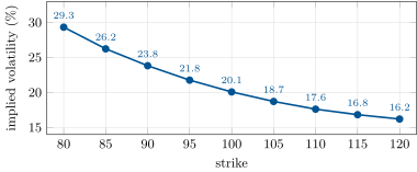
The volatility skew (or smile) is the dependence of implied volatility on strike for one expiry; the term structure of volatility is its dependence on expiry for a given moneyness. Together they form the volatility surface.

If the model behind the change of units were true, every strike would have the same implied volatility. For equity indices since 1987 the implied volatility of low strikes has been well above that of high strikes: crashes are more frequent and more feared than the model allows, and investors pay for protection. The skew is quoted as a difference in volatility points between two reference strikes or deltas, and traded as such (Figure 25.2).

**Figure 25.2.** The smile recovered from the screen prices of the chapter’s synthetic chain, out-of-the-money option at each strike, with the forward read from parity. The 90–110 skew is 6.2 volatility points. Data: the tutorial.

25.4 The volatility index

Definition 25.7 (Volatility index)

A volatility index is a published number that summarises the implied volatility of an index’s options for a fixed horizon, computed from option prices by a formula that uses no pricing model:

\sigma^2 \;=\; \frac{2}{T}\sum_i \frac{\Delta K_i}{K_i^2}\,\mathrm{e}^{RT}\,Q(K_i) \;-\; \frac{1}{T}\Bigl(\frac{F}{K_0}-1\Bigr)^2 ,

with $Q(K_i)$ the mid-quote of the out-of-the-money option at strike $K_i$ , $K_0$ the first strike at or below the forward $F$ , and the index equal to $100\,\sigma$ .

As of September 2026 — The index and its futures

The index. The best-known volatility index uses S&P 500 options of two expiries bracketing 30 days and interpolates their variances to a constant 30-day horizon. Only options with a non-zero bid enter, at mid-quote; going away from the money, the strip stops once two consecutive strikes have no bid. $K_0$ is the strike at or immediately below the forward, itself found from the strike where call and put prices are closest. The futures. Futures on the index have a multiplier of $1 000 and a tick of 0.05 point, $50. They settle on the Wednesday thirty days before the third Friday of the following month, against a special opening quotation of the index computed from the opening prices of the S&P 500 options that morning.

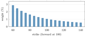
The sum weights each option by $1/K^2$ : low strikes count for more, so the index rises with the skew as well as with the general level of implied volatility. On the synthetic chain of this chapter the at-the-money volatility is 20.1 and the index-style number 23.0 (Figure 25.3). The formula is the price of the portfolio of options that replicates the variance the index will realise, a result proved in One Quant Book 5; here it matters that the index is a price of a traded portfolio, not an opinion.

The weight K/K2 given to one dollar of option premium at each strike, normalised. A dollar of premium in the 60 put counts five times as much as a dollar in the 140 call. Data: the definition. — **Figure 25.3.** The weight $\Delta K/K^2$ given to one dollar of option premium at each strike, normalised. A dollar of premium in the 60 put counts five times as much as a dollar in the 140 call. Data: the definition.

25.5 Futures on volatility

Definition 25.8 (Volatility-index future)

A VIX future is a cash-settled future on the value of the volatility index at its expiry. Since the index cannot be bought and held, the future is not tied to today’s index by a cost of carry: it is the market’s price for where the index will be.

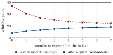
Two facts organise this market. Volatility mean-reverts, so the futures curve usually slopes up when the index is low (contango) and down when it has spiked (backwardation). And sellers of volatility are paid a premium on average: in calm periods a position short the front future earns the roll down the curve month after month, like the contango of Figure 21.3 seen from the other side.

**Figure 25.4.** Two stylised curves of futures on a volatility index. In the calm curve a short position in the first future earns 1.6 points a month if nothing happens; in the other, the market expects the index to fall by a third within three months. Illustrative numbers.

Example 25.9 (5 February 2018)

On Monday 5 February 2018 the S&P 500 fell 4% and the volatility index rose 20 points in the day. Exchange-traded products giving leveraged or inverse exposure to the front futures, with about $4 billion of assets at the end of 2017, had to rebalance at the end of the day, and, by the arithmetic of Proposition 14.10, both kinds had to buy futures after a rise. A central-bank analysis describes the resulting loop: their buying pushed the futures higher, which increased the amount they had to buy. The largest inverse product lost nearly all of its value in that session and was then terminated by its issuer.

25.6 Tutorial: from a screen of prices to a forward, a dividend and a smile

Goal. Price with the black-box formula, invert it robustly, read the forward and the implied dividend from parity, recover the smile, and compute an index-style volatility. End state: the four data figures of this chapter.

The solver. Bounds first, then bisection.

def implied_vol(premium: float, forward: float, strike: float, years: float, rate: float, right: str,
                tol: float = 1e-10) -> float:
    """Bisection on [0, 5]. Raises if the premium is outside the no-arbitrage bounds."""
    lo_price, hi_price = (price(forward, strike, years, rate, v, right) for v in (0.0, 5.0))
    if not lo_price - 1e-12 <= premium <= hi_price:
        raise ValueError(f"premium {premium} outside [{lo_price:.6f}, {hi_price:.6f}]: no implied volatility")
    lo, hi = 0.0, 5.0
    while hi - lo > tol:
        mid = 0.5 * (lo + hi)
        if price(forward, strike, years, rate, mid, right) < premium:
            lo = mid
        else:
            hi = mid
    return 0.5 * (lo + hi)

Listing 25.1. Implied volatility, or an error when no volatility can explain the price. code/firm/parity/firm_parity.py

Parity as an instrument.

def implied_forward(call: float, put: float, strike: float, years: float, rate: float) -> float:
    """Put-call parity for European options: C - P = DF (F - K)."""
    return strike + math.exp(rate * years) * (call - put)


def implied_dividends_pv(spot: float, forward: float, years: float, rate: float) -> float:
    """Present value of what the holder of the share receives (dividends) or pays (borrow fee)
    before expiry, as implied by the forward: S - DF * F."""
    return spot - math.exp(-rate * years) * forward

Listing 25.2. The forward from one strike, and the carry it implies. code/firm/parity/firm_parity.py

Reading a chain rounded to the cent, as a screen shows it.

def read_chain(rows: list[tuple[float, float, float]]):
    """From screen prices alone: the implied forward at each strike, their average, the implied
    dividend, and the implied volatility of the out-of-the-money option at each strike."""
    forwards = [implied_forward(c, p, k, YEARS, RATE) for k, c, p in rows]
    f = sum(forwards) / len(forwards)
    vols = []
    for k, c, p in rows:
        right, premium = ("P", p) if k < f else ("C", c)
        vols.append(implied_vol(premium, f, k, YEARS, RATE, right))
    return forwards, f, implied_dividends_pv(SPOT, f, YEARS, RATE), vols

Listing 25.3. Forward, dividend and smile from prices alone. code/markets-1/25-volatility-first-contact/python/vol_first.py

The strip.

def variance_strip(forward: float, years: float, rate: float, quotes: list[tuple[float, float]]) -> float:
    """Model-free implied variance from out-of-the-money option mid-quotes, in the form used by the
    best-known volatility index: (2/T) sum dK/K^2 e^{RT} Q(K) - (1/T) (F/K0 - 1)^2.
    `quotes` = (strike, mid) sorted by strike: puts below K0, calls above, their average at K0."""
    strikes = [k for k, _ in quotes]
    k0 = max(k for k in strikes if k <= forward)
    total = 0.0
    for i, (k, q) in enumerate(quotes):
        if i == 0:
            dk = strikes[1] - strikes[0]
        elif i == len(quotes) - 1:
            dk = strikes[-1] - strikes[-2]
        else:
            dk = 0.5 * (strikes[i + 1] - strikes[i - 1])
        total += dk / (k * k) * math.exp(rate * years) * q
    return 2.0 / years * total - (forward / k0 - 1.0) ** 2 / years

Listing 25.4. Model-free implied variance from out-of-the-money quotes. code/firm/parity/firm_parity.py

What to change next. Truncate the strip at 80 and 120 and see how much of the index-style volatility is lost; then widen the strike spacing from 1 to 5 and measure the discretisation error. Both are real features of published indices.

25.7 Build: parity checker and implied-volatility solver

Purpose. The first two functions every options system of the miniature firm calls: what volatility is this price, and is this chain consistent with one forward?

Interface. price(forward, strike, years, rate, vol, right); implied_vol(premium, forward, strike, years, rate, right); implied_forward(call, put, strike, years, rate); implied_dividends_pv(spot, forward, years, rate); conversion_edge(…) and reversal_edge(…) from bid and ask prices; variance_strip(forward, years, rate, quotes).

Rules. The solver raises on a premium outside the no-arbitrage bounds and never returns a negative or a clipped volatility silently. Conversions and reversals are evaluated at the prices one would actually trade: call bid and put ask for the one, the reverse for the other, with the borrow cost from Section 16.7 on the short side. Series and expiries come from the chain container (Section 23.6).

Acceptance tests. code/firm/parity/tests/: parity of the pricer; round trips of the solver across strikes and volatilities, and its refusals; a dividend recovered from a forward; conversions and reversals unprofitable inside the quotes and profitable on a planted error; the strip recovering a flat volatility to two hundredths of a point.

Stretch. American options: an early-exercise premium by a binomial tree, and the inequality form of parity.

Sources and further reading

Cboe Global Indices, Volatility Index Methodology: Cboe Volatility Index (formula, selection of options, interpolation).
Cboe Futures Exchange, VIX Futures: contract specifications.
Bank for International Settlements, “The equity market turbulence of 5 February: the role of exchange-traded volatility products”, BIS Quarterly Review, March 2018.
F. Black and M. Scholes, “The pricing of options and corporate liabilities”, Journal of Political Economy 81 (1973); F. Black, “The pricing of commodity contracts”, Journal of Financial Economics 3 (1976).

25.8 Exercises

Exercise 25.1 ★

With $r = 4\%$ and $T = 0.25$ , the 100 call is at 4.06 and the 100 put at 3.87. Give the implied forward. With the share at 100, give the implied carry.

Solution

Solution of Exercise 25.1.

$F = 100 + \mathrm{e}^{0.01}(4.06 - 3.87) = 100.19$ . Implied carry: $100 - \mathrm{e}^{-0.01} \times 100.19 = 0.81$ : an expected dividend of about eighty cents (one strike with prices rounded to the cent is good to a cent or two).

Exercise 25.2 ★

Use the at-the-money approximation to estimate the implied volatility of the 100 call of the previous exercise, and compare with the solver’s 20.1.

Solution

Solution of Exercise 25.2.

The strike is slightly below the forward, so the call is a little in the money and the put a little out: use their average, 3.965. $\sigma \approx 3.965/(0.4 \times 100.2 \times 0.990 \times 0.5) = 20.0\%$ , against 20.1 from the solver.

Exercise 25.3 ★

A volatility-index future is bought at 16.70 and sold at 19.25. Give the P&L of 40 contracts. How many ticks is that?

Solution

Solution of Exercise 25.3.

$2.55 \times \$1\,000 \times 40 = \$102\,000$ ; $2.55/0.05 = 51$ ticks.

Exercise 25.4 ★★

A three-month 90 call on a share at 100 (forward 100.20, $r = 4\%$ ) is quoted at 10.05. Show that it has no implied volatility. What should a system do with this quote?

Solution

Solution of Exercise 25.4.

The call’s lower bound is $\mathrm{e}^{-rT}(F - K) = 0.990 \times 10.20 = 10.10$ . A price of 10.05 is below it: no volatility, however small, produces it. The system must flag the quote (stale, crossed with the share, or the forward is wrong, for instance a dividend not yet in the data) and exclude it from any surface; returning zero or the previous value hides the problem.

Exercise 25.5 ★★

From a chain you read a forward of 98.10 for three months with the share at 100 and $r = 4\%$ . The company pays no dividend. Give the implied borrow fee as an annual rate and interpret it.

Solution

Solution of Exercise 25.5.

Carry $= 100 - \mathrm{e}^{-0.01} \times 98.10 = 2.88$ over a quarter: 11.5% a year. With no dividend, it is the borrow fee that the marginal arbitrageur pays to be short: the share is special, and puts look expensive against calls by exactly that amount. It is not an arbitrage for anyone who must pay the same fee.

Exercise 25.6 ★★

An index’s daily log returns over five days are $+0.4\%$ , $-1.1\%$ , $+0.7\%$ , $-2.0\%$ , $+1.5\%$ . Give the realised volatility, annualised with 252 days and without subtracting the mean. If implied volatility was 16, who was right?

Solution

Solution of Exercise 25.6.

$\sum r^2 = 0.16 + 1.21 + 0.49 + 4.00 + 2.25 = 8.11$ (in % $^2$ ); mean 1.622; daily volatility 1.274%; annualised $\times\sqrt{252}$ : 20.2%. Over these five days the buyer of options at 16 was right; five days are far too few to say more.

Exercise 25.7 ★★★

Coding. With read_chain on the chapter’s nine-strike chain report the average implied forward, the range of the nine strike-by-strike forwards, the implied dividend and the 90–110 skew. Then round prices to five cents instead of one and report the same: which numbers survive?

Solution

Solution of Exercise 25.7.

With cent prices: average forward 100.20, strike-by-strike range under three cents, implied dividend 0.80, skew 6.2 points. With five-cent prices the forward and dividend move by a few cents (the dividend estimate, 0.80, has an error of the same size as the rounding, several percent of itself) while the near-the-money volatilities barely change; the volatilities of the cheapest options, worth 0.05 to 0.35, become useless, since five cents is a large fraction of their price. Wide markets blur the wings first.

Exercise 25.8 ★★★

Find the flaw. “The volatility index is at 14 and its long-run average is 19. It is cheap: buy the front future at 15.6 and wait for mean reversion.” Use Figure 25.4.

Solution

Solution of Exercise 25.8.

The index cannot be bought; the future can, at 15.6, and the curve already contains the mean reversion: the second future is at 16.7, the seventh at 19.0. If the index stays at 14, the future bought at 15.6 converges to 14 and loses 1.6 points, $1 600 a contract, in a month, every month. Buying is a bet that the index rises faster than the curve says, against a carry that the sellers of volatility collect the rest of the time.

25.9 Problem: Reading a Chain

Problem 25.1

Weekend problem — everything the screen knows

A share trades at 100.00. Three-month European options ( $T = 0.25$ , $r = 4\%$ ) show these mid-prices:

Strike	90	95	100	105	110
Call	11.22	7.26	4.06	1.88	0.68
Put	1.12	2.11	3.87	6.63	10.38

Part I — The forward.

Compute the implied forward at each of the five strikes.
Why do they differ slightly? Which would you trust least?
Give their average.
Give the implied carry, in dollars.
The company is expected to pay 0.80 in five weeks. Is the share hard to borrow?

Part II — The smile.

Which option do you use at each strike to compute implied volatility, and why?
The solver gives 23.8, 21.8, 20.1, 18.7 and 17.6. Give the 90–110 skew and the slope in volatility points per 10% of strike.
Check the at-the-money figure with the approximation of Definition 25.4.
A colleague computes the implied volatility of the 90 call with the spot in place of the forward and finds 25.1 instead of 23.8. Explain.

Part III — Trading it.

The 100 call is bid 4.03 and offered 4.09; the 100 put 3.84 at 3.90; the share 99.99 at 100.01. With the 0.80 dividend worth 0.797 today, evaluate the conversion.
Evaluate the reversal, with a borrow cost of 0.05.
What do the two results say about the market?
A quote appears: 100 call bid at 4.60. What do you do, and what do you check first?
The next day the share is at 97 and the 100 call at 2.74. Has the call become “cheaper”? What would you compute to answer?

Part IV — Judgement.

Why do desks quote volatility and not price?
What does a skew of six points say about the market’s view of the share?
On this chain an index-style volatility would be 23.0 against 20.1 at the money. Why is it higher?
Why can implied volatility be above realised volatility on average without anyone being irrational?
State the named result: the implied dividend and the 90–110 skew.
In one sentence: what is implied volatility?

Solution

Solution of Problem 25.1.

1. $F_K = K + \mathrm{e}^{0.01}(C - P)$ : 100.20, 100.20, 100.19, 100.20, 100.20. 2. Prices are rounded to the cent and multiplied by 1.01. The least reliable are the strikes where one of the two options is far in the money: its quote is wide and it may carry an early-exercise premium if American. 3. 100.20. 4. $100 - 0.990 \times 100.20 = 0.80$ . 5. No: the implied carry equals the expected dividend (0.80, worth 0.797 today). Nothing is left over for a borrow fee. 6. The out-of-the-money option: the put below the forward, the call above. It has the tighter quote relative to its sensitivity to volatility, no intrinsic value to subtract, and no early-exercise premium to speak of. 7. $23.8 - 17.6 = 6.2$ points; 3.1 points per 10% of strike. 8. $(4.06 + 3.87)/2 = 3.965$ ; $3.965/(0.4 \times 100.2 \times 0.990 \times 0.5) = 20.0\%$ . 9. With $F = 100$ in place of 100.20 the call’s intrinsic value is understated by 0.20, so more of its 11.22 is attributed to volatility: 25.1 instead of 23.8. In-the-money options have little sensitivity to volatility, so a small error in the forward becomes a large error in implied volatility; and the call and the put at the same strike then disagree, which is the symptom to look for. 10. $4.03 - 3.90 - 100.01 + 0.797 + 99.005 = -0.08$ . 11. $3.84 - 4.09 + 99.99 - 0.797 - 0.05 - 99.005 = -0.11$ . 12. Both lose: parity holds inside the bid-ask spreads, and the chain is consistent with one forward. That is the normal state, maintained by the desks for which these two numbers are closest to zero. 13. A conversion would make $4.60 - 3.90 - 100.01 + 0.797 + 99.005 = +0.49$ a share. First check that the quote is real and current (size, exchange, time), that the share price is current, that no dividend or corporate action has changed the contract, and that the option is not about to be adjusted; then sell it. 14. Not by the price. With the dividend unchanged the forward is 97.17, and 2.74 is an implied volatility of 20.5 against 20.1 the day before: in volatility terms the call is slightly dearer. One compares volatilities, and beyond that, volatilities at comparable moneyness. 15. Because volatility is stable when the share moves, comparable across strikes, expiries and underlyings, and is the quantity a hedged option position is exposed to. 16. That the market pays more, per unit of model risk, for protection against falls than for participation in rises: fear of jumps downwards, demand for puts from holders of the share, supply of calls from overwriters. 17. It weights options by $1/K^2$ and includes the whole strip: the expensive low-strike puts count most, so the number is an average of the smile tilted towards its high side. 18. Sellers of options bear a risk that pays off badly in bad times; they are compensated by a premium, like an insurer. Implied above realised on average is that premium, and it is paid back, with interest, in months like February 2018. 19. An implied dividend of 0.80 and a 90–110 skew of 6.2 volatility points. 20. The price of an option, expressed in the one unit that stays still when the underlying moves.

25.10 Interview questions

Interview question 25.1 ★ trader, researcher

State put–call parity and say what it assumes.

Solution

Solution of Interview question 25.1.

$C - P = \mathrm{e}^{-rT}(F - K)$ for European options of the same strike and expiry. It assumes only that one can trade the forward: buy or short the underlying and borrow or lend cash. Dividends and the borrow fee enter through $F$ . No model, no distribution. For American options it becomes a pair of inequalities.

What the interviewer is looking for: model-free; the forward, not the spot; the American caveat.

Interview question 25.2 ★ trader, researcher

What is implied volatility, and why is it not a forecast?

Solution

Solution of Interview question 25.2.

The volatility that makes the Black–Scholes formula match the market price: a unit conversion. It contains the expected volatility, a risk premium for bearing it, and supply and demand for that strike; it differs by strike, which no single forecast could. On average it has exceeded subsequent realised volatility.

What the interviewer is looking for: the risk premium, and the smile as proof that it is not a forecast.

Interview question 25.3 ★★ developer, researcher

Write an implied-volatility solver. What can go wrong?

Solution

Solution of Interview question 25.3.

Check the premium against its bounds (discounted intrinsic and the discounted forward or strike) and refuse outside them. Use the out-of-the-money option via parity. Bisection always converges; Newton is faster but fails where vega is tiny, deep in or out of the money, so safeguard it with brackets. Beware: wrong forward (dividends), American premium, expiry-day options with $T \to 0$ , prices of one tick where the answer spans twenty volatility points, and time conventions (calendar or business time).

What the interviewer is looking for: bounds check, vega collapse, and the forward as the main source of error.

Interview question 25.4 ★★ trader, researcher

Calls look cheap relative to puts at the same strike. What are the possible explanations before you call it an arbitrage?

Solution

Solution of Interview question 25.4.

A dividend I have not included, or a larger one than I assumed. A borrow fee: hard-to-borrow shares have low forwards. The interest rate I use. American exercise: the put carries an early-exercise premium. Stale or wide quotes compared at mid. An expected corporate action changing the deliverable. Only when the conversion or reversal is profitable at the prices I can actually trade, including borrow, is it an arbitrage.

What the interviewer is looking for: dividends and borrow before anything else.

Interview question 25.5 ★★ researcher, trader

How is a volatility index computed, and why can you not buy it?

Solution

Solution of Interview question 25.5.

From out-of-the-money index options of two expiries bracketing thirty days: each expiry’s variance is a sum of mid-quotes weighted by $\Delta K/K^2$ , with a small correction for the distance between the forward and the nearest strike; the two variances are interpolated to thirty days, and the index is a hundred times the square root. It is the price of a portfolio that would have to be rebalanced continuously and whose composition changes every moment; one can trade futures and options on it, which price its future value, not the index itself.

What the interviewer is looking for: the strip and its weights; futures are not the index.

Interview question 25.6 ★★★ trader, researcher

Explain what happened to short-volatility products in February 2018, and what a risk manager should have seen beforehand.

Solution

Solution of Interview question 25.6.

Products short the front volatility futures had earned the roll for years and grown large. They rebalance daily to constant leverage: after a rise in the futures, both inverse and leveraged-long products must buy, in the last minutes, an amount proportional to the move. On 5 February a 4% fall in the index raised the futures; the required purchases were large relative to the futures’ liquidity, pushed the futures up further, and an inverse product lost nearly everything in a session. Visible beforehand: the products’ size relative to futures volume, the convexity of the rebalancing rule (demand grows with the move), the concentration of that demand at one time of day, and a position whose worst day exceeds its total historical profit.

What the interviewer is looking for: the rebalancing arithmetic and size relative to liquidity, not just “volatility spiked”.

Terms defined in this chapter

See all 2333 terms in the glossary