Markets I: The Ecosystem and Exchange-Traded Markets · Markets

15Index Construction and Rebalancing

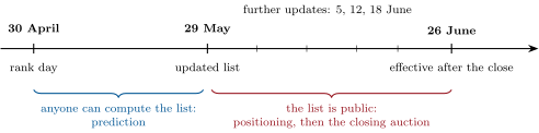
At the close of 30 April 2026 nothing visible happened: the capitalisation of every listed American company was written down. Eight weeks later, after the close of 26 June, the funds that follow one family of indices all traded to the list that snapshot had produced, in the same stocks, in the same direction, in the same auction. Everyone had known the rule for a year and the list for a month. An index is a published algorithm with a calendar, and a very large amount of money has promised to obey it. This chapter reads the algorithm as a trader does: what will have to be bought, by whom, when, and how much of the consequence is already in the price.

15.1 An index is a rulebook

Definition 15.1 (Index methodology)

An index methodology is the published document that determines an index: the universe of eligible securities, the selection rule, the weighting rule, the calendar of reviews and the treatment of corporate actions. Selection is rules-based when the document alone determines the members, and committee-based when a committee chooses among the eligible.

Definition 15.2 (Float adjustment)

Float adjustment weights each member by its capitalisation multiplied by a float factor, the fraction of its shares in the free float (Definition 8.2), so that the index can be held by everyone at once.

Definition 15.3 (Reconstitution and rebalance)

An index reconstitution is a scheduled review at which the membership is redetermined. A rebalance updates the weights (share counts, float factors, caps) of an unchanged membership. Both follow a fixed sequence: a rank day on which the data are frozen, an announcement, and an effective date, after whose close the new index applies.

Definition 15.4 (Pro-forma index)

A pro-forma index is the index as it will stand after a coming review, members and share counts, distributed by the provider to its clients between the announcement and the effective date so that trackers can prepare their trades.

As of September 2026 — Two ways of choosing five hundred or two thousand stocks

Rules-based. The Russell US indices rank companies by total capitalisation on a rank day. From 2026 they reconstitute twice a year. June 2026: rank day 30 April, preliminary lists updated on 29 May and 5, 12 and 18 June, effective after the close of Friday 26 June; the breakpoint between the large-capitalisation Russell 1000 and the small-capitalisation Russell 2000 was $5.7 billion, 24% higher than a year before. December 2026, the first December reconstitution in more than three decades: rank day 30 October, preliminary lists 13 November, effective after the close of 11 December. The provider puts the assets benchmarked to or invested in products based on these indices at about $12.2 trillion.

Committee-based. The S&P 500’s members are chosen by a committee among companies that meet published criteria. Since 1 July 2025 an addition needs a total capitalisation of at least $22.7 billion (the guideline is reviewed each quarter and set near the 85th percentile of cumulative market capitalisation), a float-adjusted capitalisation of at least half that threshold, and a ratio of annual value traded to float-adjusted capitalisation of at least 0.75, besides tests of profitability and domicile. The criteria are for additions, not for continued membership.

**Figure 15.1.** The June 2026 reconstitution of a rules-based index family (dates from the dated box). Prices after the rank day do not change the membership; they change only how much the trackers will have to buy.

15.2 Buffers

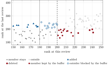
A pure “top $n$ by capitalisation” rule makes the stocks near rank $n$ enter and leave at every review. Each change costs the trackers a trade, so providers damp the rule.

Definition 15.5 (Buffer rule)

A buffer rule gives incumbents an advantage at the boundary: with a buffer $b$ , a current member of a top- $n$ index remains while it ranks $n+b$ or better, and a non-member enters only when it ranks $n-b$ or better; any places left are filled by rank. Providers express $b$ in ranks, in percentiles of cumulative capitalisation, or as a percentage band around the breakpoint.

**Figure 15.2.** One simulated review of a top-200 index with a buffer of 20 ranks (thin lines), for the stocks now ranked 150 to 250. Between ranks 180 and 220 history decides: members stay, outsiders wait. Data: the tutorial’s simulation.

**Figure 15.3.** Average number of additions per annual review of a simulated top-200 index from a universe of 600, against the width of the buffer. The number above each point is the one-way turnover in percent of index weight. A buffer of 30 ranks halves the number of changes. Data: the tutorial’s simulation, 20 paths of 20 years.

Method 15.6 (Predicting a rules-based reconstitution)

Universe. Rebuild the eligible universe from the methodology: listing venue, domicile, minimum price and float, share classes.
Capitalisation. Compute total capitalisation as the provider does, with all share classes and the latest share counts from filings. Most prediction errors are share-count errors.
Rank and band. Rank, locate the breakpoints, apply the buffer to current members.
Before the rank day, give each boundary stock a probability from its distance to the breakpoint and its volatility over the days that remain.
Size the trade with Proposition 15.7.

15.3 What the trackers must do

Proposition 15.7 (Passive demand)

Let funds with assets $A$ replicate a float-adjusted index of total float-adjusted capitalisation $M$ . They hold the same fraction $\varphi = A/M$ of the float of every member. When a stock with float-adjusted capitalisation $F$ is added they must buy $\varphi F$ dollars of it, that is a fraction $\varphi$ of its float (more precisely $AF/(M+F)$ , the difference being negligible for one addition).

Proof. A tracker holds each member at its index weight $F_i/M$ , hence $AF_i/M$ dollars of member $i$ , which is the fraction $A/M$ of $F_i$ . ∎

Definition 15.8 (Demand shock)

A demand shock is a change in the quantity of a security that some investors must hold for reasons unrelated to its value. An index change is the cleanest example: the quantity, the date and the identity of the buyers are known, and the buyers’ benchmark is the closing price of the effective date, so they are indifferent to the price they pay at that close.

Example 15.9 (Thirteen days of volume)

An index has $M = \$5$ trillion and trackers with $A = \$2$ trillion, so $\varphi = 40\%$ . A company with 400 million shares at $50, of which 65% float, has $F = \$13$ billion: a weight of 0.26% and a demand of $5.2 billion. It trades $400 million a day: the trackers need thirteen average days of volume, at one close.

Proposition 15.10 (The funding trade)

When an addition takes weight $w$ in the index, every surviving member’s weight is multiplied by $1-w$ : trackers sell $Aw_iw$ of member $i$ , and $Aw$ in total less the value of what is deleted.

Example 15.11 (One large addition)

On 16 November 2020 a provider announced that a company large enough to weigh more than one percent would join its flagship 500-stock index. It consulted the market on whether to add it in one step or two, and on 30 November announced a single step, at full float-adjusted weight, effective before the open of Monday 21 December, the pro-forma files being distributed after the close of 11 December. With $A = \$10$ trillion and $w = 1.5\%$ (round numbers, not the provider’s) the trackers would buy $150 billion of one stock and sell $9 billion of a member weighing 6%, all at one close: that of Friday 18 December, the third Friday of the month and so a quarterly expiry of index futures and options, among the most liquid closes of the year (Chapter 13).

15.4 The index effect, and where it went

Definition 15.12 (Index effect)

The index effect is the abnormal return of a stock between the announcement of its addition to (or deletion from) an index and the effective date, together with its partial reversal afterwards.

If investors held a flat demand curve for each stock, a demand shock that carries no information would not move the price. For decades it did: a study of additions to the S&P 500 finds an average abnormal return of 7.4% in the 1990s. The same study finds 0.3% for 2010–2020, and for deletions a large negative return in the 1990s against 0.1% in the later decade, although the assets tracking the index had multiplied in between. The title of the study is its conclusion: the effect has disappeared from the announcement window.

Three explanations, not exclusive. Prediction: additions are now anticipated, so the price adjusts before the announcement, where an event study does not look. Migration: many additions to the large index come from the provider’s mid-capitalisation index, whose trackers sell what the large index’s trackers buy. Liquidity supply: a population of firms now exists to buy ahead and sell to the trackers at the close. The demand shock has not disappeared; its price has been competed down, and moved earlier.

Figure 15.4. A stylised addition, in cumulative abnormal return: a jump at the announcement (day

-5

), a run-up to the effective close, a partial reversal. Only the two heights at day 0 are published averages; the shapes, the split between permanent and temporary parts and the speed of the reversal are illustrative.

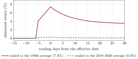
Index events remain a business (One Quant Book 8 gives the strategy files) because the averages hide a wide cross-section: small-capitalisation reconstitutions with demands of several days’ volume, migrations, float and share-count changes that nobody announces in a headline, and indices in markets where fewer firms do the arithmetic.

15.5 Tutorial: a reconstitution with buffers

Goal. Reconstitute a top- $n$ index with a buffer, measure what the buffer saves, and size the trackers’ demand. End state: the three data figures of this chapter.

The rule. Keep members inside $n+b$ , admit outsiders inside $n-b$ , then fill or trim to exactly $n$ .

def reconstitute(caps: np.ndarray, member: np.ndarray, n: int, buffer: int) -> np.ndarray:
    """Top-n index with a buffer: a member stays while ranked n + buffer or better; an outsider
    enters only when ranked n - buffer or better; remaining places are filled by rank."""
    rk = ranks(caps)
    keep = member & (rk <= n + buffer)
    enter = ~member & (rk <= n - buffer)
    new = keep | enter
    for i in np.argsort(rk):                     # fill, or trim, to exactly n names
        if new.sum() >= n:
            break
        new[i] = True
    for i in np.argsort(-rk):
        if new.sum() <= n:
            break
        if new[i] and not (member[i] and rk[i] <= n):
            new[i] = False
    return new

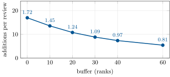
Listing 15.1. A top-

n

reconstitution with a buffer of

b

ranks. code/markets-1/15-index-construction-and-rebalancing/python/index_recon.py

Turnover. Simulate 600 lognormal capitalisations with 35% annual volatility and review once a year (Figure 15.3).

Demand.

def passive_demand(tracked_assets: float, index_cap: float, stock_float_cap: float) -> float:
    """Dollars that trackers must buy of an addition: tracked assets times its new weight."""
    return tracked_assets * stock_float_cap / index_cap


def adv_multiple(demand: float, adv_dollars: float) -> float:
    return demand / adv_dollars

Listing 15.2. What the trackers must buy, in dollars and in days of volume. code/markets-1/15-index-construction-and-rebalancing/python/index_recon.py

What to change next. Replace the rank buffer by a band of $\pm 2.5\%$ of cumulative capitalisation around the breakpoint and compare the turnover. Then give each boundary stock a probability of crossing between today and the rank day, from its volatility, and check the calibration of your probabilities over the simulated years.

15.6 Build: the reconstitution predictor

Purpose. The miniature firm’s event book (One Quant Book 8) starts from a list: which names will enter and leave, and how many days of volume the trackers will need in each.

Interface. Security(symbol, shares, price, float_factor, adv_shares, member); predict(universe, n, buffer) returning members, additions and deletions; weights(universe, members), float-adjusted; tracker_trades(universe, prediction, tracked_assets) returning for each addition and deletion the dollars, the shares and the multiple of average daily volume.

Rules. Ranking on total capitalisation, weighting on float-adjusted capitalisation: the two are different on purpose. Ties are broken by symbol so that the output is deterministic. Share counts come from the corporate-action adjuster (Section 8.7).

Acceptance tests. code/firm/recon/tests/: a five-stock universe by hand, with and without a buffer; float-adjusted weights; the trades of the trackers in an addition and a deletion.

Stretch. Crossing probabilities before the rank day; migrations between two indices of the same family with different tracked assets.

Sources and further reading

FTSE Russell, FTSE Russell begins June 2026 semi-annual Russell US Indexes reconstitution and FTSE Russell announces December 2026 Russell US Indexes reconstitution schedule, press releases, 2026.
S&P Dow Jones Indices, Update to S&P Composite 1500 Market Cap Guidelines, press releases of 4 January 2023 and 1 July 2025; S&P Dow Jones Indices Announces Implementation of Tesla’s Addition to S&P 500, 30 November 2020.
R. Greenwood and M. Sammon, “The disappearing index effect”, Journal of Finance 80 (2025), 657–698.

15.7 Exercises

Exercise 15.1 ★

A company has 400 million shares at $50; its founder holds 35% and the rest floats. Give its float-adjusted capitalisation and its weight in an index whose float-adjusted capitalisation is $5 trillion.

Solution

Solution of Exercise 15.1.

Total capitalisation $20 billion; float-adjusted $20 \times 0.65 = \$13$ billion; weight $13/5\,000 = 0.26\%$ .

Exercise 15.2 ★

Funds with $2 trillion track that index. What fraction of every member’s float do they hold? The company of the previous exercise is added and trades $400 million a day. Give the demand in dollars and in days of volume.

Solution

Solution of Exercise 15.2.

$\varphi = 2/5 = 40\%$ of every member’s float. Demand: $0.40 \times 13 = \$5.2$ billion, thirteen days of volume.

Exercise 15.3 ★

A top-100 index has a buffer of 10 ranks. Decide the fate of: a member now ranked 108; an outsider ranked 95; an outsider ranked 88; a member ranked 112.

Solution

Solution of Exercise 15.3.

Member at 108: stays ( $108 \le 110$ ). Outsider at 95: does not enter (it needs 90 or better), unless places remain to be filled by rank. Outsider at 88: enters. Member at 112: deleted.

Exercise 15.4 ★★

In the June 2026 reconstitution of Box 15.1 a company is ranked just above the $5.7 billion breakpoint on the rank day and loses 30% of its value in May. In which index is it on 29 June? What has the fall changed for the funds tracking that index, and for a firm that bought the stock in April expecting their purchases?

Solution

Solution of Exercise 15.4.

In the large index: membership was fixed on 30 April, and later prices do not change it. The fall changes the size of everything: the stock enters with a weight and a tracker demand 30% smaller in dollars (the same number of shares, since trackers hold a fraction $\varphi$ of the float). The firm that bought in April was right about the event and lost 30% on the stock: an index position is a position in the stock first. The event’s few percent cannot pay for unhedged exposure to the company.

Exercise 15.5 ★★

With the round numbers of Example 15.11, verify the two dollar amounts. What is the 6% member’s new weight? Why might the provider have considered two steps, and what is the argument for one?

Solution

Solution of Exercise 15.5.

$10\,000 \times 1.5\% = \$150$ billion. The 6% member becomes $6\% \times 0.985 = 5.91\%$ : a sale of $0.09\% \times 10\,000 = \$9$ billion. Two steps would halve the trade at each close and the strain on liquidity; but each step is a separate event to be anticipated, the index would hold a half-weight that represents nothing for a week, and trackers would bear tracking decisions twice. One step on the most liquid close available concentrates the liquidity where the demand is.

Exercise 15.6 ★★

Apply the square-root rule of Method 2.6 with $\kappa = 0.7$ and a daily volatility of 2.5% to the demand of thirteen days’ volume of Example 15.9, as if it were executed in one day. Then suppose anticipating firms buy the same quantity evenly over the twenty days before and hand it over at the close: estimate the impact of each of their days. Compare with the two averages quoted in this chapter.

Solution

Solution of Exercise 15.6.

One day: $0.7 \times 2.5\% \times \sqrt{13} = 6.3\%$ , the order of the 7.4% measured in the 1990s (and the rule is being used far outside its range). Spread over twenty days: $0.7 \times 2.5\% \times \sqrt{13/20} = 1.4\%$ a day of temporary impact, by participants who then hold the shares at risk for weeks; competition between them, and the supply from the index the stock leaves, bring the visible effect down towards the 0.3% of the last decade. The same demand, absorbed by a longer and more crowded queue.

Exercise 15.7 ★★★

Coding. With simulate_turnover(600, 200, b, 20, 1) report the additions per review and the one-way turnover for $b = 0$ and $b = 30$ . An index fund pays 15 basis points on what it trades; what does the buffer save its investors per year, in basis points of assets?

Solution

Solution of Exercise 15.7.

$b = 0$ : 18.5 additions per review, one-way turnover 1.92%. $b = 30$ : 9.2 additions, 1.18%. The fund trades twice the one-way turnover; the saving is $2 \times 0.74\% \times 15$ basis points $= 0.22$ basis point a year. Explicit costs are not the reason for buffers: the names that flip at the boundary are the smallest in the index. What buffers reduce is the number of predictable events in which trackers pay impact that the 15 basis points do not capture.

Exercise 15.8 ★★★

Find the flaw. “Buying every announced addition to the large index at the next open and selling at the effective close earned 5% per event in my backtest on 1990–2000. There are about twenty-five events a year. I expect 125% a year, unlevered.” Give three independent reasons why the expectation is wrong.

Solution

Solution of Exercise 15.8.

(i) The effect measured on that decade has since fallen to a few tenths of a percent: the backtest period is the hypothesis. (ii) The 5% was measured from prices at which a small study could trade; every participant now buys at the announcement, so the next open already contains the move, and twenty-five events do not have unlimited capacity. (iii) Returns per event do not add to an annual return: events overlap, capital is tied for days to weeks, the positions carry unhedged stock risk far larger than the edge, and costs were ignored. One may add that many additions are now predicted before they are announced, which moves the return outside the window traded.

15.8 Problem: Reconstitution Day

Problem 15.1

Weekend problem — one small stock on the last Friday of June

A small-capitalisation index has a float-adjusted capitalisation of $3 trillion and trackers with $200 billion. A large-capitalisation index of the same family has $50 trillion and trackers with $4 trillion. Stock X (price $24, float-adjusted capitalisation $1.2 billion, average volume 0.9 million shares a day, daily volatility 3%) is to join the small index. Stock Y (price $60, float $9 billion, average volume 2.5 million shares) migrates from the small index to the large one.

Part I — The demand.

What fraction of each member’s float do the small index’s trackers hold? And the large index’s?
Give the trackers’ demand for X in dollars and in shares.
Express it in days of average volume.
For Y, give the small trackers’ sale, the large trackers’ purchase and the net.
Express the sale and the net in days of Y’s volume. Which number matters for the closing price?

Part II — The close.

Trackers send 60% of their demand for X to the closing auction. X’s closing auction normally trades 8% of a day’s volume. Compare.
Estimate the impact of the whole demand for X with the square-root rule, $\kappa = 0.7$ , as if it arrived in one day.
Same if spread evenly over twenty days.
Who sells 2 million shares of X in the auction, and where did they get them?

Part III — The anticipation trade. Three weeks before the rank day a firm believes X will be added with probability 0.8. If added, it expects a run-up of 3% to the effective close; if not, a fall of 2% as other anticipators leave. A round trip costs 40 basis points. It buys $5 million.

Give the expected return and the expected profit.
Give the standard deviation of the profit.
The firm holds 25 such positions. With independent outcomes, give the expected profit, its standard deviation and their ratio.
Same with a pairwise correlation of 0.3 between the positions’ returns.
At what probability of addition does the trade break even?
Name two sources of that correlation.

Part IV — Judgement.

The provider moves from one reconstitution a year to two. What happens to the size of each event and to the anticipators’ business?
Why do the trackers accept to pay the impact at the close instead of buying early?
An index fund’s manager does buy early. Who bears the risk, and how would its investors find out?
State the named result: the trackers’ demand for X as a multiple of its average daily volume.
In one sentence: what is the economic function of the firms that anticipate index changes?

Solution

Solution of Problem 15.1.

1. $200/3\,000 = 6.67\%$ ; $4\,000/50\,000 = 8\%$ . 2. $6.67\% \times 1.2$ billion $= \$80$ million; 3.33 million shares. 3. 3.7 days. 4. Sale $6.67\% \times 9 = \$600$ million; purchase $8\% \times 9 = \$720$ million; net $+\$120$ million. 5. The sale is 4.0 days of volume, the net 0.8 day. If both groups trade in the same closing auction only the net presses on the price: a migration is mostly a cross between two sets of trackers. 6. 2 million shares against a normal auction of 72 000: 28 times. 7. $0.7 \times 3\% \times \sqrt{3.7} = 4.0\%$ . 8. $0.7 \times 3\% \times \sqrt{3.7/20} = 0.9\%$ a day. 9. The anticipators, who bought over the preceding weeks from ordinary sellers at a rate the market could bear, and market makers who go short into the auction and buy back in the following days. The auction’s imbalance feed (Chapter 13) tells them how much is still missing. 10. $0.8 \times 3\% - 0.2 \times 2\% - 0.4\% = 1.6\%$ : $80 000. 11. The return is 3% or $-2\%$ : standard deviation $\sqrt{0.8 \times 0.2} \times 5\% = 2\%$ , $100 000, before any ordinary stock risk. 12. $2 million, $500 000, ratio 4.0. 13. Standard deviation $100\,000 \times \sqrt{25 + 600 \times 0.3} = \$1.43$ million; ratio 1.4. 14. $p = (0.4\% + 2\%)/5\% = 0.48$ . 15. All the positions are long small stocks near one breakpoint: a market move before the rank day moves the breakpoint and all the probabilities together; and the same anticipators hold all the names, so when one of them reduces risk every position falls at once. 16. Each event moves fewer names and smaller weights, since half as much drift accumulates between reviews; there are twice as many dates. The total to be traded falls somewhat (fewer stocks wander far from their index), and the business becomes less seasonal and less concentrated on one Friday. 17. They are judged on tracking error against an index computed at that close. Buying early at a better price is a gain of a few basis points if it works and an unexplainable deviation if it does not. 18. The fund’s investors, through tracking error in both directions; they find out from the tracking difference in the annual report, and from nothing else. 19. 3.7 days of average volume. 20. They are the warehouse that turns a one-minute demand into a three-week one, and their profit is the fee for that.

15.9 Interview questions

Interview question 15.1 ★ trader, researcher

A stock is added to a major index. What happens to its price, and when?

Solution

Solution of Interview question 15.1.

Trackers must buy a known fraction of its float at the effective close. Historically the stock jumped at the announcement and rose into the effective date, with a partial reversal. For the large US index the measured announcement effect has gone from several percent in the 1990s to almost nothing: the move now happens earlier, as additions are predicted, and the demand is met by firms that position in advance and by the trackers of the index the stock leaves.

What the interviewer is looking for: the timeline (prediction, announcement, effective close), and knowledge that the textbook effect has shrunk.

Interview question 15.2 ★ researcher, developer

Why are indices float-adjusted, and what breaks if they are not?

Solution

Solution of Interview question 15.2.

An index is meant to be holdable by everyone simultaneously. With full capitalisation weights, trackers would need shares that a founder or a state will never sell: for a company 80% held by its founder, a demand five times larger relative to the tradable shares than for its neighbours, a squeeze at every inflow, and a price distorted by the index itself.

What the interviewer is looking for: the “everyone at once” argument and a concrete squeeze.

Interview question 15.3 ★★ researcher, trader

Trackers hold 8% of an index. A stock with a $10 billion float is added. How much must they buy? What else do you need to know to say whether that is a lot?

Solution

Solution of Interview question 15.3.

$8\% \times 10$ billion $= \$800$ million. Whether it is a lot depends on the stock’s daily volume (one day or fifteen), on the size of its closing auction, on whether it leaves another index with trackers of its own (the net, not the gross, matters), and on how much has already been bought by anticipators, which the run-up and the short interest of the auction will show.

What the interviewer is looking for: the fraction-of-float shortcut and the net of migration.

Interview question 15.4 ★★ researcher

How would you predict next June’s additions to a rules-based small-cap index, and where would your errors come from?

Solution

Solution of Interview question 15.4.

Rebuild the provider’s universe and its total capitalisations from the methodology; rank; locate the breakpoints and apply the bands to current members; before the rank day attach a crossing probability to each boundary name from distance and volatility. Errors: share counts (multiple classes, recent issues, filings the provider reads differently), eligibility details (domicile, minimum float, listing), the breakpoints themselves moving with the market, and corporate actions between rank day and effective date.

What the interviewer is looking for: share-count humility and the moving breakpoint.

Interview question 15.5 ★★ researcher, trader

Passive assets have grown enormously, yet the measured index effect has shrunk. Reconcile.

Solution

Solution of Interview question 15.5.

The measured effect is the return in a window that starts at the announcement. More passive assets mean a larger demand, but also a larger reward for predicting and supplying it: the price adjusts before the window, more capital competes to be the seller at the close, and many additions migrate from a sister index whose trackers are natural sellers. The shock grew; its price fell.

What the interviewer is looking for: the distinction between the demand and the measured return.

Interview question 15.6 ★★★ trader, researcher

You run an index-rebalance book. Describe its main risks and how you would size positions.

Solution

Solution of Interview question 15.6.

Risks: prediction error (the name is not added); stock risk between entry and the close, which dwarfs the edge and must be hedged by sector and size; crowding, visible as correlated drawdowns of all candidates when a competitor de-risks; breakpoints moving with the market; rule changes by the provider; and execution in one auction. Sizing: by days of volume to exit, not by dollars; by the probability-weighted edge net of hedging cost; with a cap on the share of the expected tracker demand that the book may hold, since beyond some share the book is its own exit.

What the interviewer is looking for: hedging of the stock leg, crowding, and sizing in units of liquidity.

Terms defined in this chapter

See all 2333 terms in the glossary