Strategies I: Equities and Futures · Strategies
14Intraday Machine-Learned Alphas
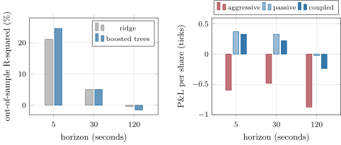
A gradient-boosted model trained on fourteen hours of a simulated order book predicts the next five seconds of the mid-price with an out-of-sample R-squared of 25%, the next thirty seconds with 5%, and the next two minutes not at all. Traded naively (crossing the spread on every forecast of a fifth of a tick or more) the five-second model loses 0.6 ticks a share: the spread it pays is larger than the moves it predicts. Traded passively, joining the queue on the forecast’s side and waiting to be filled, the same forecasts earn about a third of a tick a share. An intraday alpha is a prediction and an execution rule together; neither is worth anything alone. The build is firm.intraml.
14.1 Targets and horizons
Definition 14.1 (Intraday alpha, prediction horizon)
An intraday alpha is a forecast of a security’s price change over seconds to hours, built from market data (the order book, the trades, related securities) and traded within the day. Its prediction horizon is the interval over which the price change is forecast, which sets how often the alpha trades and what execution cost it can bear.
The target of this chapter is the change of the mid-price over the next 5, 30 and 120 seconds, in ticks, sampled every second on twenty one-hour sessions of firm.tape (Book 7, chapter 2), whose default configuration includes a news window in mid-session. Its spread is about one tick (1.07 on average) and the standard deviation of the target is 0.69 ticks at five seconds, 2.19 at thirty and 4.47 at two minutes. Kolm, Turiel and Westray, forecasting 115 Nasdaq stocks at several horizons, found that stock-specific forecasts had an effective horizon of about two average price changes: beyond that, the book says little. The synthetic tape agrees in shape.
14.2 Features from the book and the tape
Ten features, all computed from data up to the forecast’s second (Listing 14.1): the top-of-book imbalance, the spread, the order-flow imbalance of Cont, Kukanov and Stoikov over the last 1, 5 and 30 seconds (Book 7, chapter 8), the signed trade volume over 5 and 30 seconds (Book 7, chapter 9), the mid’s own change over 5 and 30 seconds, and the microprice’s distance from the mid. Order-flow features, normalised by the book’s depth, are the ones the literature finds stationary: Kolm and co-authors report that models trained on order flow outperform most models trained on raw book states. The unit tests check causality by construction: cutting the tape at a time leaves every feature before it unchanged.
14.3 Models and their validation
Two models per horizon: ridge regression on the standardised features, and a gradient-boosted ensemble (Friedman’s method) of sixty depth-two regression trees split on quantiles of the features, written in a few dozen lines of NumPy. Training uses sessions 1 to 14 and testing sessions 15 to 20: whole sessions apart, so that overlapping targets (a thirty-second target at second shares 29 seconds with the one at ) cannot leak across the split, the purging and embargo of Book 7, chapter 20 at session scale.
| horizon | 5 seconds | 30 seconds | 120 seconds |
|---|---|---|---|
| out-of-sample R-squared: ridge; boosted trees | 21.1%; 24.6% | 5.1%; 5.1% | ; |
| rank IC: ridge; boosted trees | 0.33; 0.34 | 0.23; 0.28 | 0.07; 0.07 |
| in-sample R-squared, boosted trees | 23.3% | 9.2% | 3.2% |
| every forecast above 0.2 ticks, aggressive (ticks a share) | |||
| every forecast above 0.2 ticks, passive | 0.37 | 0.33 | |
| coupled: aggressive above the spread, passive below | 0.33 | 0.22 |
The five-second R-squared of a quarter is high by the standard of real markets, and the reason is the tape: Book 7 found that its mids trend over a few seconds, a property the chapter’s model learns. What carries over is the pattern across horizons (a rapid decay of predictability, with the thirty-second forecast already down to 5% and the two-minute one worthless out of sample while it still fits 3.2% in sample) and the small gain of the trees over ridge where there is a signal to find. Sirignano and Cont found, with deep learning on billions of US quotes, that a model trained on all stocks predicts better than stock-specific ones, even for stocks outside its training set: price formation from order flow is largely universal. That is an argument for pooling data across instruments, which this chapter’s twenty sessions only mimic.
14.4 Coupling the alpha to execution
Definition 14.2 (Execution coupling)
Execution coupling is the design of an intraday strategy’s orders from its forecast: crossing the spread only when the forecast exceeds the cost of crossing, resting passively when it does not, and sizing and cancelling orders as the forecast changes, so that the alpha and the execution are one decision.
The table’s lower half is the chapter’s point. A forecast of a fifth of a tick does not pay a spread of a tick: crossing on every such forecast loses 0.60 ticks a share at five seconds. The same forecasts, used to choose which side of the book to join, earn 0.37 ticks a share on the orders that are filled (Listing 14.2), because a passive order earns the spread instead of paying it and the forecast tilts the fills toward the favourable side. Coupling the two (crossing only when the forecast exceeds the spread, 324 times over six test hours, and resting otherwise) earns 0.33 ticks a share at five seconds and 0.22 at thirty. At two minutes nothing works: the forecast has no out-of-sample power, and both execution styles lose. The passive numbers are optimistic in one way (the fill model fills a resting order as soon as the market trades through its price, ignoring its place in the queue; Book 7, chapter 18 has the queue-aware replay) and honest in another (the exit crosses the spread).
s1_intraml.14.5 Strategy files
Strategy file 14.1 — Book-imbalance alpha
Who pays you, and why. Traders whose orders reveal pressure before prices move: the book’s imbalance is the queue that will be eaten next.
Instruments and venues. Liquid stocks and futures with deep, visible books.
Signal. Top-of-book and depth imbalance, order-flow imbalance over seconds.
Sizing and execution. Mostly passive, joining the favoured side; aggressive only when the forecast beats the spread.
Costs. Spread, fees and rebates; queue position.
How it dies. Faster competitors reading the same book; spoofed depth.
Horizon, capacity, infrastructure. Seconds; small capacity per name; co-located, low-latency systems.
Backtest honestly. A queue-aware replay (Book 7, chapter 18); latency; fees.
Sources. Cont, Kukanov and Stoikov (2014); this chapter’s simulation.
Strategy file 14.2 — Trade-flow alpha
Who pays you, and why. Metaorders split into many trades, whose signs persist (Book 7, chapter 9).
Instruments and venues. As for book imbalance.
Signal. Signed trade volume over seconds to minutes; the persistence of trade signs.
Sizing and execution. As for book imbalance.
Costs. As for book imbalance.
How it dies. Metaorders that hide better; competitors on the same flow.
Horizon, capacity, infrastructure. Seconds to minutes; the trade feed with its sign.
Backtest honestly. Trade signs as they could be known (Lee–Ready or the feed’s aggressor flag), with its latency.
Sources. Kolm, Turiel and Westray (2023) on order-flow inputs.
Strategy file 14.3 — Cross-asset lead alpha
Who pays you, and why. Slower instruments that follow faster ones (a stock after its index future, an ETF after its constituents).
Instruments and venues. Pairs of related instruments on the same or different venues.
Signal. The leader’s recent move, relative to the follower’s (Book 7, chapter 10).
Sizing and execution. Trade the follower in the leader’s direction before it catches up.
Costs. Speed: the gain is only there for whoever is first.
How it dies. Latency competition; the lead shrinking to microseconds.
Horizon, capacity, infrastructure. Milliseconds to seconds; networks and co-location (Books 10 and 11).
Backtest honestly. Timestamps from the same clock; realistic latency between venues.
Sources. Sirignano and Cont (2019) on universal, pooled features; no performance figure verified.
Strategy file 14.4 — Alpha-driven execution
Who pays you, and why. The spread, earned instead of paid, when the forecast chooses where to rest.
Instruments and venues. Any instrument the firm trades for other reasons, and market-making books.
Signal. The short-horizon forecast, against the spread and the queue.
Sizing and execution. Aggressive above the spread, passive below, cancel when the forecast turns.
Costs. Adverse selection on passive fills; cancellation limits.
How it dies. It does not die; it saves cost on every other strategy’s trading.
Horizon, capacity, infrastructure. Seconds; an execution engine that takes forecasts as input.
Backtest honestly. Queue-aware fills; the markouts of passive fills (Book 7, chapter 23).
Sources. This chapter’s simulation (0.33 ticks a share coupled against aggressive at five seconds).
14.6 Tutorial: one per cent is a lot
Goal. Build features from the synthetic tape, train and validate two models at three horizons, and trade their forecasts three ways. End state: the table and Figure 14.1.
Features: every second, from data up to that second.
def features(tape, step: float = 1.0):
    top = tape.top
    t = top["t"]
    bid, ask = top["bid"].astype(float), top["ask"].astype(float)
    bq, aq = top["bid_qty"].astype(float), top["ask_qty"].astype(float)
    e = np.zeros(len(t))                                          # order-flow imbalance increments
    e[1:] = ((bid[1:] >= bid[:-1]) * bq[1:] - (bid[1:] <= bid[:-1]) * bq[:-1]
             - (ask[1:] <= ask[:-1]) * aq[1:] + (ask[1:] >= ask[:-1]) * aq[:-1])
    ce = np.cumsum(e)
    tr = tape.trades
    cf = np.concatenate([[0.0], np.cumsum(tr["sign"] * tr["qty"].astype(float))])
    times = np.arange(30.0, tape.cfg.seconds - 1e-9, step)
    i = _at(t, times)
    mid = 0.5 * (bid + ask)

    def lag(k, arr):
        return arr[i] - arr[_at(t, times - k)]

    def flow(k):
        return cf[np.searchsorted(tr["t"], times, side="right")] - cf[np.searchsorted(tr["t"], times - k, side="right")]

    depth = np.maximum(bq[i] + aq[i], 1.0)
    X = np.column_stack([(bq[i] - aq[i]) / depth, ask[i] - bid[i], lag(1, ce) / depth, lag(5, ce) / depth,
                         lag(30, ce) / depth, flow(5) / depth, flow(30) / depth, lag(5, mid), lag(30, mid),
                         (bid[i] * aq[i] + ask[i] * bq[i]) / depth - mid[i]])
    return times, X, NAMES, mid[i]
Listing 14.1. Order-book and trade-flow features. code/firm/intraml/firm_intraml.py Passive execution: join the touch on the forecast’s side; filled only if traded through; exit across the spread.
def passive(tape, times, pred, h: float, threshold: float, wait: float = 10.0):
    """Join the touch in the forecast's direction; filled if a trade prints through the price within `wait`; exit across
    the spread h seconds after the fill."""
    top, tr = tape.top, tape.trades
    tt = top["t"]
    out = []
    for k in np.flatnonzero(np.abs(pred) > threshold):
        t0 = times[k]
        i = _at(tt, t0)
        side = 1 if pred[k] > 0 else -1
        px = top["bid"][i] if side > 0 else top["ask"][i]
        a, b = np.searchsorted(tr["t"], t0, side="right"), np.searchsorted(tr["t"], t0 + wait, side="right")
        hit = np.flatnonzero((tr["sign"][a:b] == -side) & (side * (tr["price"][a:b] - px) <= 0))
        if len(hit) == 0 or tr["t"][a + hit[0]] + h > tape.cfg.seconds:
            continue
        j = _at(tt, tr["t"][a + hit[0]] + h)
        exit_px = top["bid"][j] if side > 0 else top["ask"][j]
        out.append(side * (exit_px - px))
    return np.array(out, float)
Listing 14.2. Passive entries with a touch-fill model. code/firm/intraml/firm_intraml.py - Run
scores(h),naive(h)andtrading(h)for 5, 30 and 120 seconds, andfig_intraml.py.
What to change next. Replace the touch-fill model by Book 7’s queue-aware replay; add the second instrument of simulate_pair as a lead feature; train one model on all horizons with the horizon as a feature.
14.7 Build: intraday machine learning
Purpose. Causal intraday features, horizon targets, two models with session-level validation, and execution rules coupled to the forecasts.
Interface. features(tape, step), targets(tape, times, horizons), ridge and ridge_predict, gbm and gbm_predict, r2(y, yhat), aggressive(pred, fwd, spread, threshold), passive(tape, times, pred, h, threshold, wait).
Rules. Features from data up to each time; training and test separated by whole sessions; costs in every P&L.
Acceptance tests. code/firm/intraml/tests/: features unchanged when the future is removed; both models recover a planted signal; the aggressive P&L by hand.
Stretch. A queue-aware passive fill model; cross-asset features; deeper trees and early stopping on a validation session.
Sources and further reading
- R. Cont, A. Kukanov and S. Stoikov, “The price impact of order book events”, Journal of Financial Econometrics 12(1), 2014.
- P. N. Kolm, J. Turiel and N. Westray, “Deep order flow imbalance”, Mathematical Finance 33(4), 2023.
- J. Sirignano and R. Cont, “Universal features of price formation in financial markets”, Quantitative Finance 19(9), 2019.
- J. H. Friedman, “Greedy function approximation: a gradient boosting machine”, Annals of Statistics 29(5), 2001.
14.8 Exercises
Exercise 14.1 ★
A forecast has an R-squared of 25% against a target with a standard deviation of 0.69 ticks. What is the standard deviation of the forecast?
Solution
Solution of Exercise 14.1.
The correlation is , so a well-calibrated forecast has a standard deviation of ticks: most forecasts are a third of a tick or less, well below a one-tick spread.
Exercise 14.2 ★
Why can a thirty-second target at second not be validated on a sample that contains second ?
Solution
Solution of Exercise 14.2.
The two targets share 29 of their 30 seconds, so a model tested on second after training on second has seen almost all of the test target: the test measures memory, not prediction. Training and test must be separated by at least the horizon (purging and an embargo), here by whole sessions.
Exercise 14.3 ★
An aggressive round trip pays one spread of a tick. What must a forecast predict, in ticks, to break even?
Solution
Solution of Exercise 14.3.
One spread: a forecast of at least a tick in the direction traded, before fees.
Exercise 14.4 ★★
Why do passive fills earn money on forecasts too small to pay the spread? What biases the chapter’s passive numbers upward?
Solution
Solution of Exercise 14.4.
A passive order earns the spread when it is filled; the forecast chooses the side that the price is more likely to move toward, so fills are less adversely selected than random fills. The fill model is optimistic: it fills the order as soon as the market trades through its price, as if it were at the front of the queue.
Exercise 14.5 ★★
The two-minute model fits 3.2% in sample and out of sample. What happened?
Solution
Solution of Exercise 14.5.
It fitted noise: with little signal at two minutes, the trees found patterns in the training sessions that do not recur, and the forecast adds variance without predictive power, so the out-of-sample R-squared is below zero.
Exercise 14.6 ★★
Why normalise order-flow features by the book’s depth?
Solution
Solution of Exercise 14.6.
The same order flow moves the price more when the book is thin: dividing by depth makes the feature comparable across times and instruments and closer to stationary, as Cont, Kukanov and Stoikov’s linear relation with a slope inversely proportional to depth suggests.
Exercise 14.7 ★★★
Coding. Train the models with the mid’s own past changes removed from the features, and compare the five-second R-squared. What does the difference say about the synthetic tape?
Solution
Solution of Exercise 14.7.
Without the mid’s past changes the five-second R-squared is 18.6% for ridge (against 21.1%) and 24.4% for the trees (against 24.6%): almost nothing is lost. The order-flow and imbalance features already contain the short-term trend, which on the synthetic tape is driven by the flow itself.
Exercise 14.8 ★★★
Find the flaw. “Our model predicts the next second’s price change with 60% accuracy on direction; we will trade it with market orders on 3 000 stocks.”
Solution
Solution of Exercise 14.8.
Direction accuracy says nothing about the size of the moves against the spread: a one-second forecast is worth a fraction of a tick and a market order pays half a spread in and half out. It must be traded passively or not at all, and the accuracy must be measured out of sample with realistic latency.
14.9 Problem: One Per Cent Is a Lot
Problem 14.1
Weekend problem — a forecast and its execution
The chapter’s models on firm.tape, and the published record.
Part I — The forecast.
- Define an intraday alpha and its prediction horizon.
- Describe the targets, the sessions and the spread.
- List the features and how causality is tested.
- What did Kolm, Turiel and Westray find about horizons and inputs?
Part II — The models.
- Describe the two models.
- How are training and test separated, and why by session?
- Give the out-of-sample R-squared and IC by horizon.
- Why is the five-second R-squared so high here?
Part III — Execution.
- Define execution coupling.
- Give the P&L per share of the three execution styles by horizon.
- Why do aggressive trades lose on small forecasts?
- What does the passive fill model assume?
Part IV — The verdict.
- State the named result: out-of-sample R-squared by horizon and the P&L per share after the spread, aggressive against passive.
- What did Sirignano and Cont find about universality?
- How would you pool data across instruments?
- What would change with a queue-aware replay?
- How does latency enter?
- Which strategy file is least exposed to competition?
- What is the capacity of a five-second alpha?
- In one sentence: what is an intraday alpha worth?
Solution
Solution of Problem 14.1.
- A seconds-to-hours forecast built from market data and traded within the day; the interval over which the move is forecast.
- The mid’s change over 5, 30 and 120 seconds, every second, in twenty one-hour sessions; a spread of about 1.07 ticks.
- Imbalance, spread, order-flow imbalance over 1, 5 and 30 seconds, signed volume over 5 and 30, own returns over 5 and 30, microprice distance; features must not change when the future is removed.
- Order-flow inputs beat raw book states; the effective horizon is about two average price changes.
- Ridge regression and sixty depth-two boosted trees.
- Training on sessions 1–14, testing on 15–20, so overlapping targets cannot leak.
- 21.1% and 24.6% at 5 seconds, 5.1% at 30, below zero at 120; ICs 0.33–0.34, 0.23–0.28, 0.07.
- The synthetic tape’s mids trend over a few seconds, driven by its order flow.
- Choosing the order type and price from the forecast: cross only when the forecast beats the spread.
- Aggressive , , ; passive 0.37, 0.33, ; coupled 0.33, 0.22, ticks a share.
- The spread they pay exceeds the moves they predict.
- Fills as soon as the market trades through the order’s price: front of the queue.
- Named result. Out-of-sample R-squared of 24.6%, 5.1% and at 5, 30 and 120 seconds (boosted trees); after the spread, aggressive trading of every forecast loses 0.60 ticks a share at five seconds while passive entries earn 0.37 and the coupled rule 0.33.
- A single model trained on all stocks predicts better than stock-specific ones, even out of sample in stocks it has not seen.
- Normalise features and targets by each instrument’s tick, spread and depth, and train one model on all of them.
- Passive fills would be fewer and more adversely selected; the passive and coupled P&L would fall.
- The forecast decays within seconds, so a delay in data or orders eats the part that is predictable.
- Alpha-driven execution, which saves costs on trades the firm makes anyway.
- Small: a fraction of the size at the touch, in each name.
- What it saves or earns after the spread, in the execution it is designed with.
14.10 Interview questions
Interview question 14.1 ★ researcher, mle
What features would you build from an order book to predict the next few seconds?
Solution
Solution of Interview question 14.1.
Top-of-book and depth imbalance, order-flow imbalance over several windows, signed trade volume, the spread, the microprice’s distance from the mid, recent returns, and the same for related instruments; all normalised by depth or volatility.
Interview question 14.2 ★★ researcher, mle
How do you cross-validate a model whose targets overlap in time?
Solution
Solution of Interview question 14.2.
Split in time with a gap at least as long as the horizon (purging) and a further embargo, or by whole sessions; never shuffle; report walk-forward results.
Interview question 14.3 ★★ trader
Your model predicts moves smaller than the spread. Is it useless?
Solution
Solution of Interview question 14.3.
No: use it to decide where to rest passive orders and when not to, which earns or saves part of the spread; it becomes useless only if even passive fills are adversely selected beyond what the forecast recovers.
Interview question 14.4 ★★ mle, developer
How would you serve a gradient-boosted model within microseconds of a market data update?
Solution
Solution of Interview question 14.4.
Flatten the trees into arrays of thresholds and leaf values, update features incrementally from each message, keep everything in cache, and evaluate in compiled code (C++ or Rust) without allocation; or precompute lookup tables for the features’ quantiles.
Interview question 14.5 ★★ researcher
Why might an R-squared of 1% be a good intraday model?
Solution
Solution of Interview question 14.5.
Because it is traded thousands of times a day in many instruments: a small edge per trade, if it survives costs, adds up; and returns at short horizons are mostly noise, so a 1% R-squared can mean a correlation of 0.1, a large information coefficient.
Interview question 14.6 ★★★ researcher
A forecast of a move has correlation with it and both are normal with standard deviations and . With a round-trip cost , derive the expected P&L per trade of trading only when , and discuss how it depends on .
Solution
Solution of Interview question 14.6.
Given , . Trading when earns per trade; with normal, , so the P&L grows linearly with and is positive only when times that tail mean exceeds : a weak correlation needs a high threshold, and trades rarely.